Introduction to MLE: How to Automatically Learn Parameters with Code (A Sample of Machine Learning)

2025-07-27 ｜ Research ｜ #Words: 4252 ｜中文原版

Maximum Likelihood Estimation (MLE), also translated as “maximum likelihood estimation”, is a method for obtaining the optimal parameters of a model from sample data.

For example, MLE can estimate the parameters of a probability density function (PDF). If a set of samples/datasets/statistics (likely) follow a normal distribution, we only need to find the mean and variance (or standard deviation) of the dataset to derive the probability density formula that fits the data.

\[f(x) = \frac{1}{\sqrt{2\pi\sigma^2}} e^{-\frac{(x - \mu)^2}{2\sigma^2}}\]

Where:

$\mu$ represents the mean
$\sigma^2$ represents the variance
$x$ is the value of the random variable

The Process of Maximum Likelihood Estimation

The steps for MLE are as follows:

Determine the probability model: e.g., a normal distribution model.
Construct the likelihood function: this involves multiplying all probability density functions together.

Alternatively, we can convert it to a logarithmic function, which turns the product into a sum—this is more convenient in some cases. Additionally, addition is computationally cheaper than multiplication for computers.
As an extra note: although the function itself is continuous, the probability density function becomes “discrete” when applied to discrete samples, which is why we can multiply them together. You’ll see this clearly in the code later.
Solve for the maximum value of the log-likelihood function

For each data point, we substitute the current $x$ value into the function (e.g., the standard normal distribution function), where the parameters are the independent variables of the likelihood function. We then take the derivative to find the optimal MLE parameters.
For program implementation, the derivative tells us the direction of parameter adjustment.

Demonstrating How Machines Learn Parameters via MLE

You might have found this article while studying for an exam, but once you understand the principle of MLE, it mostly comes down to memorizing formulas. So instead, we’ll demonstrate how to estimate parameters using code.

Let’s arbitrarily choose parameters for a normal distribution PDF: $\mu = 7.2$, $\sigma = 2.8$ (which means $\sigma^2 = 7.83999$).

We’ll start with the standard normal distribution (you can start with other values) and iteratively adjust the parameters until they match our target parameters (referred to as such below).

First, we generate 10,000 data points using the target parameters as our sample data, then fit the parameters from this sample.

The key differences from exam-style problem-solving are: 1) We need to find two parameters instead of just one, and 2) We won’t use direct differentiation to find the values.

Below are key code snippets (see comments for explanations)—the full code is provided later:

    def __init__(self):
        # Target distribution parameters
        self.target_mu = 7.2    # Theoretical mean
        self.target_sigma = 2.8 # Theoretical standard deviation
        self.target_var = self.target_sigma **2  # Theoretical variance
        
        # MLE estimated parameters
        self.mle_mu = 0.0       # Mean estimate
        self.mle_sigma = 1.0    # Standard deviation estimate
        self.mle_var = self.mle_sigma** 2  # Variance estimate

Next, generate the data:

    def generate_data(self, n_samples=100000):
        """Generate observed data"""
        self.data = np.random.normal(
            loc=self.target_mu,
            scale=self.target_sigma,
            size=n_samples
        )
        print(f"Generated {n_samples} data points from N(μ={self.target_mu}, σ²={self.target_var:.2f})")
        
        # Theoretical MLE values (sample statistics)
        # Note: sample statistics differ slightly from theoretical values (shown later)
        self.true_mle_mu = np.mean(self.data)
        self.true_mle_var = np.var(self.data, ddof=0)
        self.true_mle_sigma = np.sqrt(self.true_mle_var)
                
        return self.data

Now we can perform maximum likelihood estimation:

    def mle_gradient_descent(self, epochs=10000, lr=0.05, tol=1e-8):
        # No separate test set available, so manually split into train/validation sets
        # This is a common technique
        train_data, val_data = train_test_split(self.data, test_size=0.2, random_state=42)
        
        # Initialize parameters to starting values
        self.mle_mu = self.initial_mu
        self.mle_var = self.initial_var
        self.mle_sigma = np.sqrt(self.mle_var)
        
        # Variables for tracking training progress and plotting
        self.train_log_likelihoods = []
        self.val_log_likelihoods = []
        self.epochs_record = []
        best_val_ll = -np.inf
        best_mu, best_var = self.mle_mu, self.mle_var
        
        # Counter for overfitting prevention (early stopping)
        counter = 0 
        
        # Start training
        for epoch in range(epochs):
            # Convert to logarithmic scale for easier calculation
            # loc=self.mle_mu: location parameter (mean)
            # scale=np.sqrt(self.mle_var): scale parameter (standard deviation)
            # After logarithmic conversion, we sum log-probability densities (cheaper addition)
            # Note: Values closer to 0 indicate better fitting to training data
            train_ll = np.sum(stats.norm.logpdf(train_data, loc=self.mle_mu, scale=np.sqrt(self.mle_var)))
            val_ll = np.sum(stats.norm.logpdf(val_data, loc=self.mle_mu, scale=np.sqrt(self.mle_var)))
            
            # Record values for plotting
            self.train_log_likelihoods.append(train_ll)
            self.val_log_likelihoods.append(val_ll)
            self.epochs_record.append(epoch + 1)
            
            # Difference between training set and estimated mean
            error = train_data - self.mle_mu 
            # Calculate gradient for mean
            grad_mu = np.mean(error / self.mle_var)
            # Squared error between training set and estimated variance
            mean_squared_error = np.mean(error **2)
            # Calculate gradient for variance
            grad_var = (-1/(2*self.mle_var)) + (mean_squared_error)/(2*self.mle_var** 2)
            
            # Update parameters: adjust by (learning rate * gradient)
            self.mle_mu += lr * grad_mu
            self.mle_var += lr * grad_var
            # Variance cannot be negative (set to 0 if negative)
            self.mle_var = max(self.mle_var, 0) 
            # Calculate standard deviation (used for early stopping)
            # We originally defined the target in terms of standard deviation (not variance)
            self.mle_sigma = np.sqrt(self.mle_var)
            
            # Early stopping (stop if validation loss worsens for 50 consecutive epochs)
            if val_ll > best_val_ll:
                best_val_ll = val_ll
                best_mu, best_var = self.mle_mu, self.mle_var
                counter = 0
            else:
                counter += 1
                if counter >= 50 or (abs(val_ll - best_val_ll) < tol):
                    print(f"\nConverged at epoch {epoch+1}")
                    self.mle_mu, self.mle_var = best_mu, best_var
                    self.mle_sigma = np.sqrt(self.mle_var)
                    break
            
            # Print training progress every 100 epochs
            if (epoch + 1) % 100 == 0:
                print(f"Epoch {epoch+1}/{epochs} - "
                      f"Train LL: {train_ll:.2f}, Val LL: {val_ll:.2f}, "
                      f"MLE Mean: {self.mle_mu:.4f}, MLE Variance: {self.mle_var:.4f}")
        
        return self.train_log_likelihoods

Let’s explain this section of the code:

# Calculate gradient for mean
grad_mu = np.mean(error / self.mle_var)
# Squared error between training set and estimated variance
mean_squared_error = np.mean(error **2)
# Calculate gradient for variance
grad_var = (-1/(2*self.mle_var)) + (mean_squared_error)/(2*self.mle_var** 2)

In computer science, gradients and derivatives are often implemented using their basic definition: rate of change. Unlike mathematical derivatives (which involve limits), real-world implementations are simpler (as seen in the code). However, you still need to manually calculate the derivative for the variance gradient.

First, the log-likelihood function is: $\log L(\mu, \sigma^2) = -\frac{n}{2}\log(2\pi) - \frac{n}{2}\log(\sigma^2) - \frac{1}{2\sigma^2}\sum_{i=1}^n (x_i - \mu)^2$

Take the partial derivative with respect to $\sigma^2$ (note: $\sigma^2$, not $\sigma$): $\frac{\partial \log L}{\partial \sigma^2} = -\frac{n}{2\sigma^2} + \frac{1}{2\sigma^4}\sum_{i=1}^n (x_i - \mu)^2$

Factor out $\frac{n}{2\sigma^2}$: $\frac{\partial \log L}{\partial \sigma^2} = \frac{n}{2\sigma^2} \left( \frac{\sum (x_i - \mu)^2}{n\sigma^2} - 1 \right)$

The factor $n$ doesn’t affect the calculation (it’s just a constant coefficient), so we can omit it to reduce computations: $\frac{\partial \log L}{\partial \sigma^2} = \frac{1}{2\sigma^2} \left( \frac{\sum (x_i - \mu)^2}{n\sigma^2} - 1 \right)$

While $\mu$ represents the mathematical expectation (mean) in theory, we use the sample-calculated mean in practice.

This is a critical concept: the learning rate must be consistent for all parameters. As you’ll see in training, the mean converges much faster than the variance (due to the squared term in variance calculations). Using different learning rates for each parameter will result in significant estimation errors.
Try it yourself—you’ll see the final parameters have huge errors.
Is there a solution? Yes—modern models often use variable learning rates (e.g., reducing the learning rate when loss decreases slowly to improve accuracy) or learning rate schedules. However, this is beyond the scope of this article and won’t be discussed further.

We can now start training.

Below is the complete code—you can copy and run it yourself:

import numpy as np
import pandas as pd
import matplotlib.pyplot as plt
from scipy import stats
from sklearn.model_selection import train_test_split
import os
import time 

np.random.seed(42)

class MLENormalEstimator:
    def __init__(self):
        self.target_mu = 7.2 
        self.target_sigma = 2.8 
        self.target_var = self.target_sigma **2 
        
        self.initial_mu = 0.0
        self.initial_sigma = 1.0
        self.initial_var = self.initial_sigma** 2
        
        self.mle_mu = self.initial_mu
        self.mle_sigma = self.initial_sigma
        self.mle_var = self.initial_var
        
    def generate_data(self, n_samples=100000):
        self.data = np.random.normal(
            loc=self.target_mu,
            scale=self.target_sigma,
            size=n_samples
        )
        print(f"Generated {n_samples} data points from N(μ={self.target_mu}, σ²={self.target_var:.2f})")
        
        self.true_mle_mu = np.mean(self.data)
        self.true_mle_var = np.var(self.data, ddof=0) 
        self.true_mle_sigma = np.sqrt(self.true_mle_var)
        
        return self.data
    
    def mle_gradient_descent(self, epochs=10000, lr=0.05, tol=1e-8):
        train_data, val_data = train_test_split(self.data, test_size=0.2, random_state=42)
        
        self.mle_mu = self.initial_mu
        self.mle_var = self.initial_var
        self.mle_sigma = np.sqrt(self.mle_var)
        
        self.train_log_likelihoods = []
        self.val_log_likelihoods = []
        self.epochs_record = []
        best_val_ll = -np.inf
        best_mu, best_var = self.mle_mu, self.mle_var
        counter = 0
        
        start_time = time.time()
        
        for epoch in range(epochs):
            train_ll = np.sum(stats.norm.logpdf(train_data, loc=self.mle_mu, scale=np.sqrt(self.mle_var)))
            val_ll = np.sum(stats.norm.logpdf(val_data, loc=self.mle_mu, scale=np.sqrt(self.mle_var)))
            
            self.train_log_likelihoods.append(train_ll)
            self.val_log_likelihoods.append(val_ll)
            self.epochs_record.append(epoch + 1)
            
            error = train_data - self.mle_mu
            grad_mu = np.mean(error / self.mle_var)
            mean_squared_error = np.mean(error **2)
            grad_var = (-1/(2*self.mle_var)) + (mean_squared_error)/(2*self.mle_var** 2)
            
            self.mle_mu += lr * grad_mu
            self.mle_var += lr * grad_var
            self.mle_var = max(self.mle_var, 0)
            self.mle_sigma = np.sqrt(self.mle_var)
            
            if val_ll > best_val_ll:
                best_val_ll = val_ll
                best_mu, best_var = self.mle_mu, self.mle_var
                counter = 0
            else:
                counter += 1
                if counter >= 50 or (abs(val_ll - best_val_ll) < tol):
                    print(f"\nConverged at epoch {epoch+1}")
                    self.mle_mu, self.mle_var = best_mu, best_var
                    self.mle_sigma = np.sqrt(self.mle_var)
                    break
            
            if (epoch + 1) % 100 == 0:
                print(f"Epoch {epoch+1}/{epochs} - "
                      f"Train LL: {train_ll:.2f}, Val LL: {val_ll:.2f}, "
                      f"MLE Mean: {self.mle_mu:.4f}, MLE Variance: {self.mle_var:.4f}")
        
        end_time = time.time()
        self.train_duration = end_time - start_time 
        
        return self.train_log_likelihoods
    
    def evaluate(self):
        print("\n" + "="*80)
        print("                  MAXIMUM LIKELIHOOD ESTIMATION RESULTS")
        print("="*80)
        print(f"1. Training Duration: {self.train_duration:.4f} seconds") 
        print(f"\n2. Target Distribution:")
        print(f"   - Mean: {self.target_mu:.6f}")
        print(f"   - Variance: {self.target_var:.6f}")
        
        print(f"\n3. Theoretical MLE (Sample Statistics):")
        print(f"   - Mean MLE: {self.true_mle_mu:.6f}")
        print(f"   - Variance MLE: {self.true_mle_var:.6f}")
        
        print(f"\n4. Estimated MLE:")
        print(f"   - Estimated Mean: {self.mle_mu:.6f}")
        print(f"   - Estimated Variance: {self.mle_var:.6f}")
        
        print(f"\n5. Initial Parameters:")
        print(f"   - Initial Mean: {self.initial_mu:.6f}")
        print(f"   - Initial Variance: {self.initial_var:.6f}")
        
        print(f"\n6. Estimation Errors:")
        print(f"   - Mean Error: {abs(self.true_mle_mu - self.mle_mu):.8f}")
        print(f"   - Variance Error: {abs(self.true_mle_var - self.mle_var):.8f}")
        print("="*80 + "\n")
        
        # Plot log-likelihood curve
        plt.figure(figsize=(6, 4))
        plt.plot(self.epochs_record, self.train_log_likelihoods, label='Training Log-Likelihood', 
                 color='blue', linewidth=1.2)
        plt.plot(self.epochs_record, self.val_log_likelihoods, label='Validation Log-Likelihood', 
                 color='orange', linewidth=1.2)
        plt.title('Log-Likelihood During MLE Optimization', fontsize=10)
        plt.xlabel('Epoch', fontsize=8)
        plt.ylabel('Log-Likelihood (Higher = Better)', fontsize=8)
        plt.grid(True, linestyle='--', alpha=0.5)
        plt.legend(fontsize=7)
        plt.tight_layout()
        plt.savefig('corrected_mle_log_likelihood.png', dpi=150)
        plt.close()
        
        # Plot distribution comparison
        plt.figure(figsize=(6, 4))
        x_min = min(self.data.min(), self.target_mu - 4*self.target_sigma, self.initial_mu - 4*self.initial_sigma)
        x_max = max(self.data.max(), self.target_mu + 4*self.target_sigma, self.initial_mu + 4*self.initial_sigma)
        x = np.linspace(x_min, x_max, 1000)
        
        plt.hist(self.data, bins=100, density=True, alpha=0.6, color='blue',
                 label=f'Observed Data (μ={self.true_mle_mu:.2f})')
        plt.plot(x, stats.norm.pdf(x, self.target_mu, self.target_sigma), 'g-', lw=2,
                 label=f'Target Distribution')
        plt.plot(x, stats.norm.pdf(x, self.mle_mu, self.mle_sigma), 'r--', lw=2,
                 label=f'Estimated MLE Distribution')
        plt.plot(x, stats.norm.pdf(x, self.initial_mu, self.initial_sigma), 'purple', ls=':', lw=1.5,
                 label=f'Initial Distribution')
        
        plt.title('Distribution Comparison', fontsize=10)
        plt.xlabel('Value', fontsize=8)
        plt.ylabel('Probability Density', fontsize=8)
        plt.legend(fontsize=7)
        plt.grid(alpha=0.3)
        plt.savefig('mle_distribution_comparison.png', dpi=150)
        plt.close()
        
        print("Generated plots:")
        print("1. corrected_mle_log_likelihood.png - Log-likelihood curve")
        print("2. mle_distribution_comparison.png - Distribution comparison (with initial curve)")

if __name__ == "__main__":
    estimator = MLENormalEstimator()
    estimator.generate_data(n_samples=100000)
    
    print("\nStarting maximum likelihood estimation...")
    estimator.mle_gradient_descent(
        epochs=10000,
        lr=0.1,
        tol=1e-8
    )
    
    estimator.evaluate()    

The output (last part shown below) will look like this:

Epoch 9600/10000 - Train LL: -195870.32, Val LL: -49077.16, MLE Mean: 7.2181, MLE Variance: 7.8367
Epoch 9700/10000 - Train LL: -195870.32, Val LL: -49077.16, MLE Mean: 7.2181, MLE Variance: 7.8368
Epoch 9800/10000 - Train LL: -195870.32, Val LL: -49077.16, MLE Mean: 7.2181, MLE Variance: 7.8368
Epoch 9900/10000 - Train LL: -195870.32, Val LL: -49077.16, MLE Mean: 7.2181, MLE Variance: 7.8368
Epoch 10000/10000 - Train LL: -195870.32, Val LL: -49077.16, MLE Mean: 7.2181, MLE Variance: 7.8369

================================================================================
                  MAXIMUM LIKELIHOOD ESTIMATION RESULTS
================================================================================
1. Training Duration: 27.8044 seconds

2. Target Distribution:
   - Mean: 7.200000
   - Variance: 7.840000

3. Theoretical MLE (Sample Statistics):
   - Mean MLE: 7.202707
   - Variance MLE: 7.854133

4. Estimated MLE:
   - Estimated Mean: 7.218075
   - Estimated Variance: 7.836873

5. Initial Parameters:
   - Initial Mean: 0.000000
   - Initial Variance: 1.000000

6. Estimation Errors:
   - Mean Error: 0.01536817
   - Variance Error: 0.01726031
================================================================================

Generated plots:
1. corrected_mle_log_likelihood.png - Log-likelihood curve
2. mle_distribution_comparison.png - Distribution comparison (with initial curve)

You can see that the “4. Estimated MLE” values are very close to both “3. Theoretical MLE (Sample Statistics)” and “2. Target Distribution”—this took only 27 seconds.

Naturally, changing the random seed will affect training outcomes.

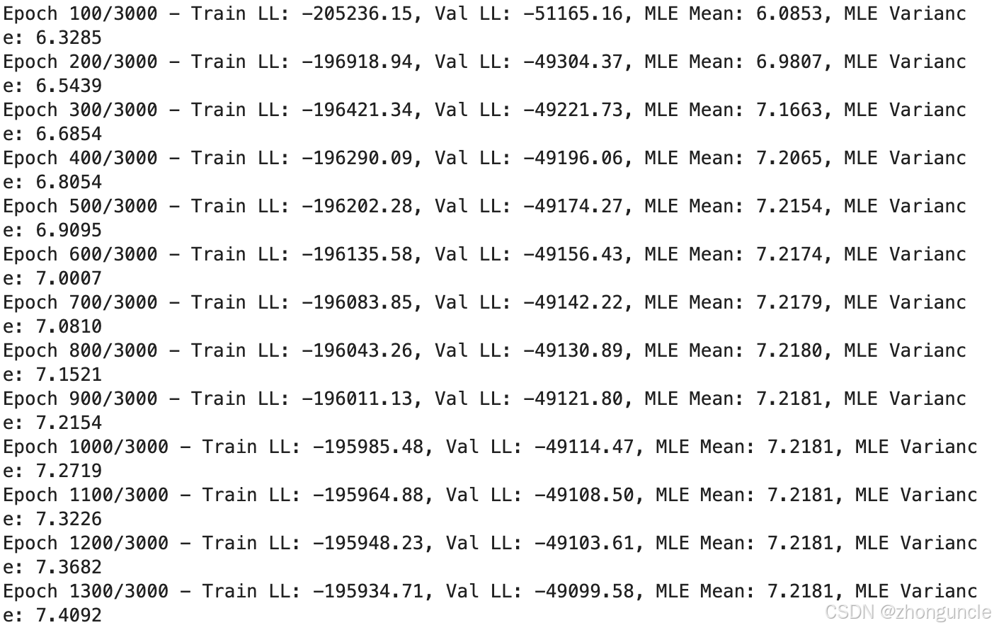
If you’re willing to sacrifice some accuracy for faster training, you can lower the epoch value. The mean (MLE Mean) stabilizes at 1000 epochs, with subsequent training focused solely on the variance (MLE Variance):

Log-likelihood curve showing mean convergence at 1000 epochs

The code includes plotting functionality that visually demonstrates the fitting results:

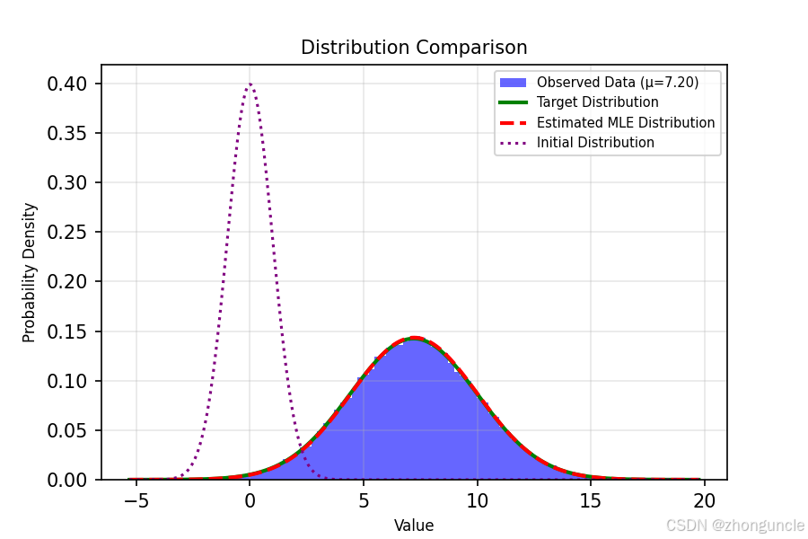
Distribution comparison: initial normal distribution, observed data, target distribution, and estimated MLE distribution

The dashed purple line on the far left is the standard normal distribution (initial state), the blue histogram is the sampled dataset (samples/statistics), the green line is the target distribution curve, and the dashed red line (appearing reddish-orange here) is our fitted MLE distribution curve—you can see they are nearly identical.

I hope these will help someone in need~