Origin, Code, Performance and Differences of QuickSort algorithms(qsort)
When I was learning quicksort algorithm, I found there are many style of code (for example, the quicksort mentioned in the textbook and online is different). I was very curious why. So I went to read “Introduction to Algorithms” to search for answer. Finally I found the reason be related to the development history of quicksort.
So I consulted a lot of materials and wrote this blog as a record.
Development history of quicksort
If you look at the chapter about quicksort in “Introduction to Algorithms”, the book will tell you that quicksort was first published in 1962 by C.A.R Hoare (Winner of the Turing Award in 1980) in the fifth volume of “The Computer Journal” First proposed in the published paper “Quicksort” (https://doi.org/10.1093/comjnl/5.1.10). However, in “Communications of the ACM” at the end of 1961, C.A.R Hoare had already given a simple explanation using the Algol 60 in “Algorithm 64: Quicksort”:
And if you check the paper “Quicksort” just mentioned, you will find that the only citation of the paper is “Algorithm 64: Quicksort” at the end of 1961, as follows:

“Quicksort” only describes this method, as well as many features and performance, and uses mathematical methods to prove the time complexity of quicksort.
So when was the quicksort algorithm invented? Now we need to talk about Mr. Hoare’s experience.
C.A.R Hoare’s full name is Charles Antony Richard Hoare. From 1952 to 1956, Mr Hoare studied Humanities (Literae Humaniores) at Merton College, Oxford. After graduation, due to the requirements of the United Kingdom at that time, I went to the Royal Navy for two years of national service. Because of his literary background in college, Hoare took a Russian course to learn modern military Russian. In 1958, Hoare returned to Oxford and began to study statistics (Statistics), and in this year, Hoare came into contact with programming (Mercury Autocode) for the first time. In 1959, Hoare attended Moscow State University as a visiting student for a year. During this period, Hoare began to use computer science technology to translate Russian literature into English because he needed to process the contents of the dictionary. However, Hoare did not understand the sorting algorithm at the time, so he rediscovered the bubble sort algorithm (Bubblesort) on his own, but felt it was too slow. He invented a second algorithm himself, so he invented the quicksort algorithm (Quicksort). In 1960 Hoare returned to England and began working.
Conclusion, Hoare invented the quicksort algorithm in 1959-1960 in order to translate Russian into English, and formally proposed the quicksort algorithm in 1962 through the paper “Quicksort”.
Then in “Programming Pearls” first published in 1986, the author mentioned that Nico Lomuto has a more concise method, which is the quicksort algorithm that appeared in “Introduction to Algorithms (Third Edition)”. Generally, It is called “Lomuto-Partition”; some textbooks show a variant of the Hoare version quicksort, it is called “Hoare-Partition”.
The next section will describe the difference between the two in detail. If you want to see more differences between other quicksort algorithms, you can read Chapter 12 of “Programming Pearls”.
Mr. Hoare’s experience references: Encyclopedia Britannica-Tony Hoare Interview: An Interview with C.A.R. Hoare
The difference between Hoare-Partition and Lomuto-Partition
Principle of quicksort algorithm
Before introducing the difference between Hoare-Partition and Lomuto-Partition, you must know the principle of the quicksort algorithm.
The principle of quicksort algorithm is:
- Select a value from the array that needs to be sorted as the “Pivot Element” (it is translated as “Pivot Element” in the introduction to the algorithm, and the word “pivot element” is used below for simplicity), This value is generally the first element on the left.
- Then use the pivot to divide the array into two sub-arrays. This process is called “Partition”. In general, any value in the subarray on the left is less than the pivot, and any value in the subarray on the right is greater than the pivot.
- Perform iterative sorting on the left and right sub-arrays.
- After iteration, you can finally get the sorted array.
Therefore, the quicksort algorithm has a template, and those that conform to the template are called “quicksort”. This template is the template in “ALGORITHM 64” that appeared before. In short, it is roughly as follows:
//quicksort(A, m, n). A is an array, m and n are integers, m represents the beginning of the array to be sorted, and m represents the end.
//Comparing m and n in condition is to prevent the sorted array from being an array with less than 2 elements, which makes no sense in sorting.
if m<n {
	partition(...)
	quicksort(...)
	quicksort(...)
}
The key is partition part, different quicksort depending on this part. So let’s first talk about the specific implementation of each method in detail, and then to compare.
First, prepare an array for testing. In order to understanding, the array is short, as follows:
int testArr[10]={6,10,8,4,2,5};
Hoare-Partition
How to implement using C
#include <stdio.h>

void myqsort(int a[], int lo, int hi);
void swap(int a[], int i, int j);
void displayArr();

int main()
{
    int num = sizeof(testArr)/sizeof(int);

    myqsort(testArr, 0, 50);
    displayArr();

	return 0;
}

int hoare_partition(int a[], int lo, int hi)
{
    int x=a[lo];

    // due to use do-while, so need +1 or -1
    int i = lo - 1;
    int j = hi + 1;

    while (i<j){
    	// Compare to Pivot x from left. if large or equal to x, finish loop
        do {
            i++;
        } while (a[i]<x);

        // Compare to Pivot x from right. if large or equal to x, finish loop
        do {
            j--;
        } while (a[j]>x);

        // In the above two loops, i and j are "running" to each other (to be precise, i comes first and j comes last)
        if (i<j){
        // If i and j have not met at this time (a[i] should be to the right of the pivot x, and a[j] should be to the left of the pivot x), then exchange the i-th and j-th elements to continue.
            swap(a, i, j);
        }else{
			// If now i==j, return j as pivot in next iteration (Also you can use i, but Hoare uses the j)
            return j;
        }
    }
    return -1;
}

void myqsort(int a[], int lo, int hi)
{
    if (lo<hi){
    	// Divide array
        int m=hoare_partition(a, lo, hi);
        // Start iteration sort
        myqsort(a, 0, m-1);
        myqsort(a, m+1, hi);
    }
}

void swap(int a[], int i, int j)
{
    int temp;
    temp=a[i];
    a[i]=a[j];
    a[j]=temp;
}

void displayArr(){
    for (int i=0; testArr[i]!=0; i++) {
        printf("%d ",testArr[i]);
    }
    printf("\n");
}
Performance test
The test platform is Mac mini 2018 i5-8500B 4.1GHz 32g+512g. The fan is adjusted to 4400 full speed using Mac Fan Control. The SSD temperature is about 40 degrees and the CPU temperature is 50~75 (Intel Power Gadget shows it is hovering between 60~80). No SSD overheating or slowing down.
The test data is 100 integers in the range of 0~1000000000(10^9). However, since it spends so long time just used the first 60 data. So I only 10~50 data are tested. According to the data and calculation formula, the 60 cases will take more than four hours (actually I tested it, CPU Time: 18241.949540s, just over five hours).
The following data is a bit outrageous. I will try to know why.
The running results on the local NVMe SSD disk:
| Number | Time |
|---|---|
| 10 | 0.000005s |
| 20 | 0.000150s |
| 30 | 0.012972s |
| 40 | 2.463117s |
| 50 | 180.790424s |
| 60 | 18241.949540s |
In USB flash drive:
| Number | Time |
|---|---|
| 10 | 0.000004s |
| 20 | 0.000188s |
| 30 | 0.012851s |
| 40 | 2.536276s |
| 50 | 183.398252s |
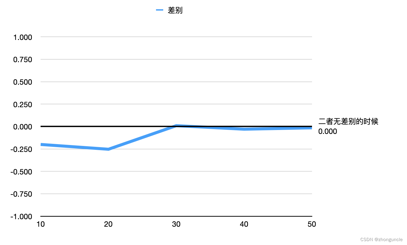
Both roughly fit the average time complexity curve: nlog_2n
The performance differences between NVMe SSD and USB flash drive are as follows:
Lomuto-Partition
How to implement using C
In order to simplify the code here, only lomuto_partition is listed. Except that you need to change the function name when declaring it, the rest is exactly the same as the previous section:
int lomuto_partition(int a[], int lo, int hi)
{
    // Set the rightmost element (highest bit) as Pivot
    int x=a[hi];
    // Set i to divide array, left part less than Pivot, right part more than Pivot
    int i = lo-1;

    // Set j with leftmost element. j is to control the bound of right part of array, so can be equal to hi
    for (int j=lo; j <= hi-1; j++) {
        //if a[j] less or equal Pivot x, add 1 to i and exchange a[i] and a[j]
        if (a[j]<=x) {
            i++;
            swap(a, i, j);
        }
    }

    // After comparing the entire array, exchange the element hi and i
    swap(a, i+1, hi);
    return i+1;
}
Performance test
The same level of testing Lomuto-Partition is much faster, as follows:
| Number | Time |
|---|---|
| 10 | 0.000002s |
| 20 | 0.000006s |
| 30 | 0.000014s |
| 40 | 0.000032s |
| 50 | 0.000058s |
Differences
Logically, “Hoare-Partition” is “run to each other, judge and exchange “; while “Lomuto-Partition” is “starting-pursuing”.
In speed, “Lomuto-Partition” is faster.
In ease of understanding, “Lomuto-Partition” is also easier. Although many people may think that “Hoare-Partition” is simpler, you can try to write it by yourself, rather than copy from Google or book. You will find “Hoare-Partition” is easier to make mistakes.
Other Quicksort
Quick sort algorithm in some textbooks
In some textbooks about data structure, you can see the following form of “partition”.
If you read it carefully, you will find it is a variant of “Hoare-Partition”. It also likes “Lomuto-Partition” sorting from both ends to the middle exchange the position of the pivot x last. But it compares one end first completely, and then compare the other end. Since using while syntax, in order to prevent overflow, th add lo<hi to condition.
int partition(int a[], int lo, int hi)
{
    int x=a[lo];
    while (lo<hi){
        while (lo<hi && a[hi]>=x){
            hi--;
        }
        if (lo<hi){
            a[lo]=a[hi];
            lo++;
        }
        while (lo<hi && a[lo]<=x){
            lo++;
        }
        if (lo<hi){
            a[hi]=a[lo];
            hi--;
        }
    }
    a[lo]=x;

    return lo;
}
The time is also between the two, closer to “Hoare-Partition”:
| Number | Time |
|---|---|
| 10 | 0.000006s |
| 20 | 0.000181s |
| 30 | 0.028264s |
| 40 | 2.305088s |
| 50 | 98.516586s |
qsort on K&R
In “The C Programming Language” known as the “K&R C Language Bible”, Brian wrote a quick sort program. However, the original text is used to compare input characters, and some C novices may not understand the concise writing without braces, so the code here has been modified.
This algorithm is one of the simplest quick sort algorithms and is also very fast. Since the logic is not much similar to what was mentioned before and looks different, we will discuss the principle after the code.
int K_R_partition(int a[], int lo, int hi)
{
int i, last;
swap(a, lo, (lo+hi)/2);
// The pivot in this algorithm is the middle element a[(lo+hi)/2] of the initial array, because the meaning of "lo" has been changed above
// Here, the initial value of lo is assigned to 'last', so that 'last' can "walk" to the right instead of lo, so that lo can maintain the value of the pivot without moving.
last = lo;
//In the initial state, i is 1 larger than 'last', that is, the part in 'last' left starts to move.
//This also illustrates that the algorithm only processes half of the array each time until the recursion reaches the minimum, and the processing is completed.
for(i = lo+1; i <= hi; i++) {
// During the loop, if a[i] is less than the pivot a[lo], swap the element at the last position with the element at the i position after adding 1 to last.
// It means put the value smaller than a[lo] to the right of a[lo], so that in the end, as long as the values of lo and last are interchanged, it can ensure that all values smaller than the pivot are on the left of the pivot
if (a[i] < a[lo]) {
swap(a, ++last, i);
}
}
// Swap the 'last' back to lo, so that all values smaller than the pivot a[lo] are on the left of the pivot a[lo]
swap(a, lo, last);
// Returns 'last' which is the pivot of this loop
return last;
}
This algorithm only arranges the second half of the array each time, and place the elements in the array that are smaller than the pivot element in the left half of the second half, so that the elements that are larger than the pivot are in the second half. Multiple iterations in this way can sort the array.
Other quick sort algorithms not listed
There are other quick sorting algorithms, such as three-number centering, fuzzy sorting, etc. Since I don’t know much about them yet, I’ll fill them in when I learn more about them later.
I hope these will help someone in need~