Verify the central limit theorem using C++

The reason why I want to write this blog is I watched But what is the Central Limit Theorem? - YouTube published the famous mathematical popularization account 3Blue1Brown. This video mention: regardless of whether the probabilities of various situations of this discrete event are average or not, when the number is certain to be large, it will still follow a normal distribution curve. I just want to try to see whether is the case. I think the central limit theorem (CLT) and normal distribution are a very magical part of probability theory.

I will use dice points as discrete events to calculate the probability of the sum of points. First, Implementing the program to simulate a uniformly distribute. Second, adjusting the probability of non-uniform distribution.

The source code in ZhongUncle/Prove-CLT-in-CPP - GitHub.

The probability of the sum of points under uniform distribution

First, create a array to store points of dices, like:

int a[] = {1,2,3,4,5,6};

Generating PPM images use the function writePPMImage:

void writePPMImage(int* data, int width, int height, const char *filename, int maxIterations)
{
    FILE *fp = fopen(filename, "wb");

    // write ppm header
    fprintf(fp, "P6\n");
    fprintf(fp, "%d %d\n", width, height);
    fprintf(fp, "255\n");

    for (int i = 0; i < width*height; ++i) {
        float mapped = pow( std::min(static_cast<float>(maxIterations), static_cast<float>(data[i])) / 256.f, .5f);
        unsigned char result = static_cast<unsigned char>(255.f * mapped);
        for (int j = 0; j < 3; ++j)
            fputc(result, fp);
    }
    fclose(fp);
    printf("Wrote image file %s\n", filename);
}

The parameters of writePPMImage:

1. data is an array where each element corresponds to the color information (Z-word arrangement) of each pixel in image. The sum of points corresponding to an element (or a pixel), there is add one to this value.
2. width and heightare the dimensions of the generated bitmap image.
3. filename is the filename of the generated bitmap image.
4. maxIterations is the maximum value of the color (white). Here set it to 256, because it is treated as an 8-channel color in the code. Or you can just write it as 1, and use integer values 0 and 1 to represent black and white.

Below, I will write the code directly. Please read the comments for the explanations of each step:

int main() {
	//set image size 1450x1000
    int width = 1450;
    int height = 1000;
    
    // choose one element as dice point 
    int a[] = {1,2,3,4,5,6};
    
    // store the result of sum of dice points. Don't declear an empty array here, because some compiler will set empty elements to "strange" value and run in error (C compiler will set 0 default)
    int* sumArr = new int[width];
    // array stored the color of pixel for output
    int* output = new int[width*height];
	
    // number of samples is 30x1000=30000, so will get 30000 sum of dice points
    for (int i=0; i<height*30; i++) {
    	// get a random point. %6 means the range of random points is 0~5, corresponding length of a[]
        int temp = a[random()%6];
        // this for will accumulate sum 100 times, it represents how much dice points add together.=
        for (int j=0; j<100; j++) {
            temp = temp + a[random()%count];
        }
	    // add 1 to corresponding value in sumArr[]
	    sumArr[temp] = sumArr[temp]+1;
    }
	    
	// the beginning of output of image is bottom, so need the conversion
	for (int i=0; i<width; i++) {
	    for (int j=height-1; j>=height-sumArr[i]; j--) {
	        output[j*width+i]=256;
	    }
	}
	// output image
	writePPMImage(output, width, height, "output.ppm", 256);
	
	delete[] sumArr;
	delete[] output;
	return 0;
}

The image generated by 30000 samples like:

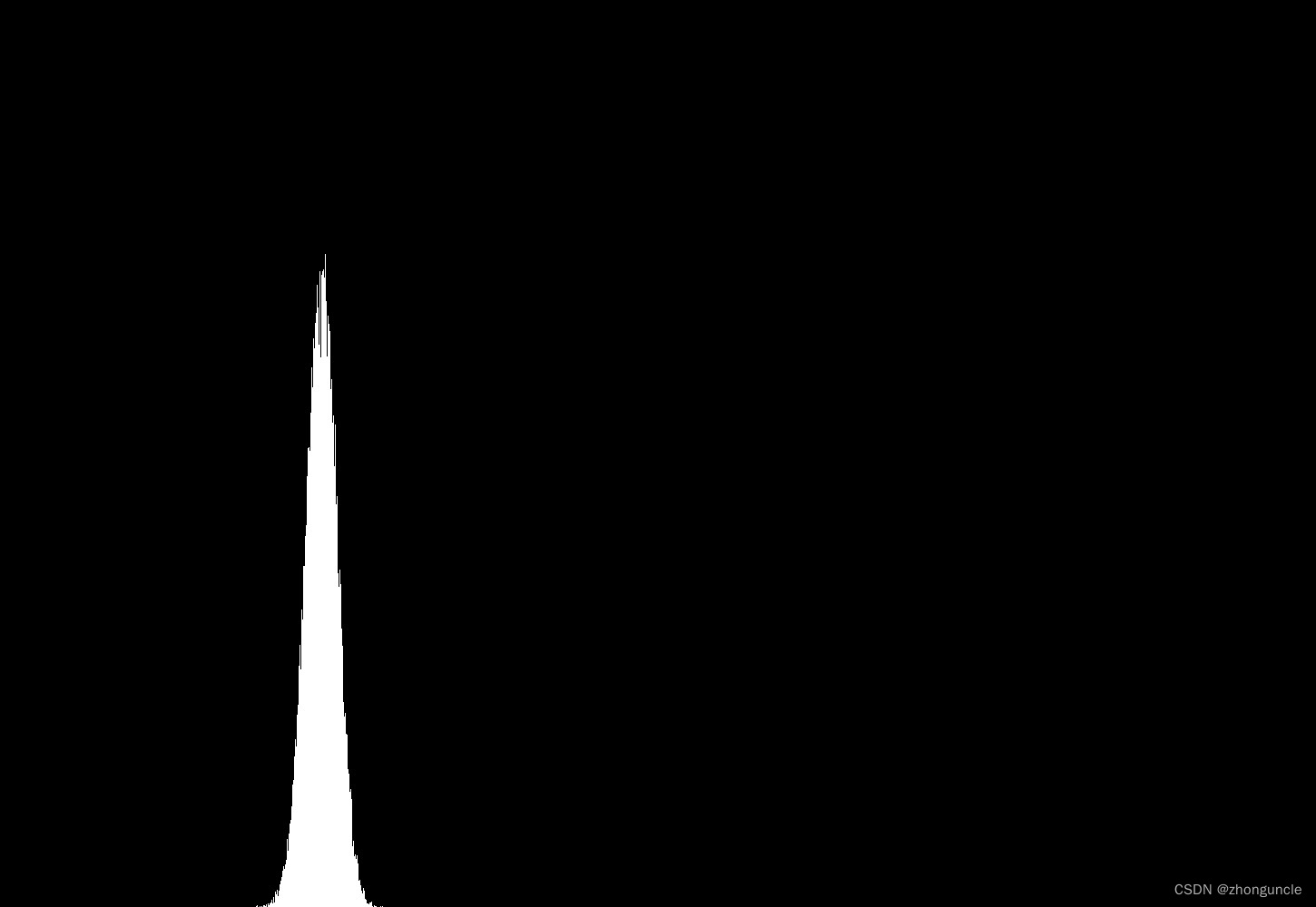
It’s little similar to the normal distribution curve, but too sharp. To make it more obvious, let’s ‘widen and flatten’ it. The method is to modify the second large ‘for’ loop as follows:

for (int i=0; i<width; i++) {
        // sumArr[i]/2 to flatten image
        for (int j=height-1; j>=height-sumArr[i]/2; j--) {
            // widening images
            for (int k=0; k<10; k++) {
                output[j*width+i*10+k]=256;
        }
    }
}

It means 2x10 pixel represent a sample, below all images use this scale. Now image likes：

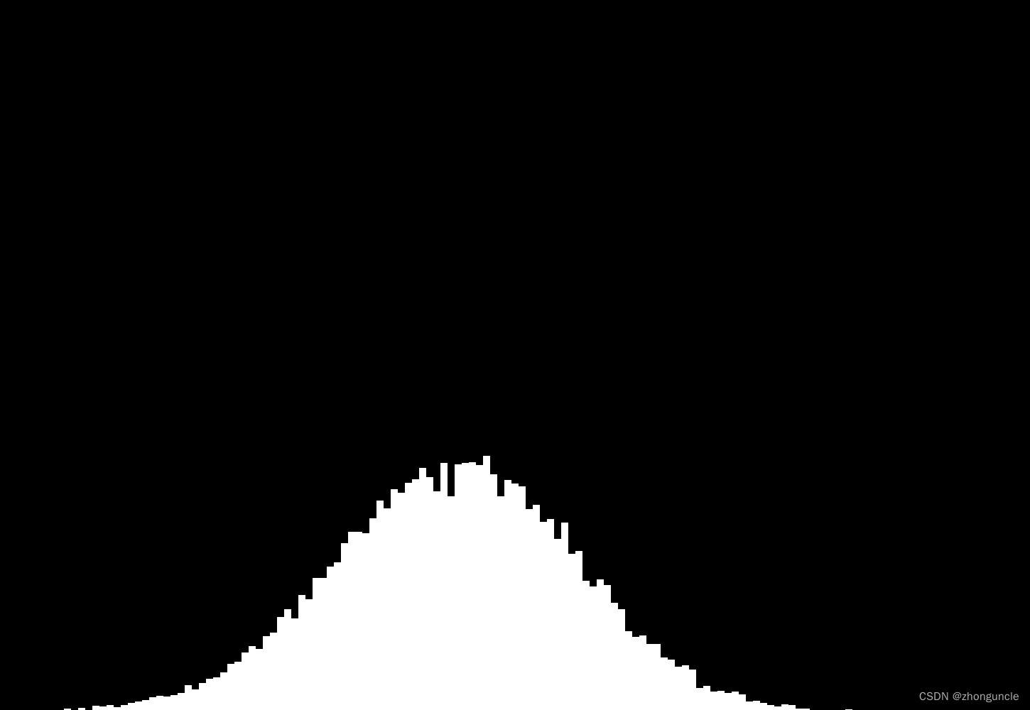
Now it’s very similar to the normal distribution curve. If you want to get a standard normal distribution curve, you just need calculate the variance and sample mean.

Probability of the sum of points under non-uniform distribution

Next, let’s try an image of the probability of non-uniform distribution.

When I start to implement it, it makes me in proble. I didn’t know how to make the probability of each value different, but quickly I realized that this likes catching small balls (elements) in the box (array). So just modifying the number of elements and values in the array is fine. The array represents the sample space is:

int a[] = {1,1,1,1,1,2,3,4,5,6};

There are five 1. It means probability of 1 is 0.5 (5/10), others are 0.1 (1/10).

At this point, it needs to modify the source code, not only because the number of elements has changed and the range of random values has also changed, but also because it needs to be written in a more general way considering various testing situations. Therefore, modify to the following:

int main() {
    int width = 1700;
    int height = 1000;
    int a[] = {1,1,1,1,1,2,3,4,5,6};
    //count is used to calculate the size of the sample space, and we don't need to manually modify
    int count = sizeof(a)/sizeof(int);
    
    
    int* sumArr = new int[width];
    int* output = new int[width*height];

    for (int i=0; i<height*30; i++) {
        int temp = a[random()%count];
        for (int j=0; j<100; j++) {
            temp = temp + a[random()%count];
        }
        sumArr[temp] = sumArr[temp]+1;
    }
    
    for (int i=0; i<width; i++) {
        // sumArr[i]/2 to flatten image
        for (int j=height-1; j>=height-sumArr[i]/2; j--) {
            // widening images
            for (int k=0; k<10; k++) {
                output[j*width+i*10+k]=256;
            }
        }
    }

    writePPMImage(output, width, height, "output.ppm", 256);

    delete[] sumArr;
    delete[] output;
    return 0;
}

Now the image gengerated like:

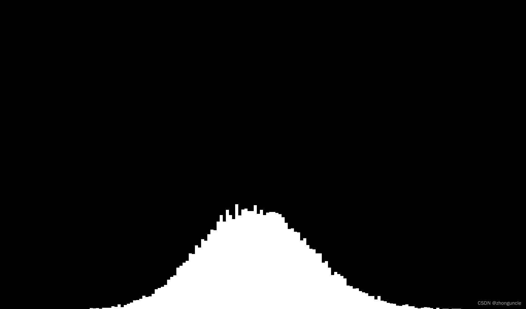
It still conforms to the normal distribution curve and not change in the image due to the higher probability of ‘1’.

What about probability greater? What if the probability of ‘1’ is as high as 99%?

Unfortunately, to achieve a probability of up to 99% for ‘1’, the sample space array will have 500 elements, which can lead to some resource allocation errors. So I try to set the probability of ‘1’ is 95%, then this array is as follows (you can copy below code and try it):

int a[] = {
       	1,1,1,1,1,1,1,1,1,1,1,1,1,1,1,1,1,1,1,1,1,1,1,1,1,1,1,1,1,1,1,1,1,1,1,1,1,1,1,1,1,1,1,1,1,1,1,1,1,1,1,1,1,1,1,1,1,1,1,1,1,1,1,1,1,1,1,1,1,1,1,1,1,1,1,1,1,1,1,1,    //#'1' = 40
        1,1,1,1,1,1,1,1,1,1,1,1,1,1,1,1,1,1,1,1,1,1,1,1,1,1,1,1,1,1,1,1,1,1,1,1,1,1,1,1,1,1,1,1,1,1,1,1,1,1,1,1,1,1,1,1,1,1,1,1,1,1,1,1,1,1,1,1,1,1,1,1,1,1,1,1,1,1,1,1,    //#'1' = 40
        1,1,1,1,1,1,1,1,1,1,1,1,1,1,1,1,1,1,1,1,1,1,1,1,1,1,1,1,1,1,1,1,1,1,1,1,1,1,1,1,1,1,1,1,1,1,1,1,1,1,1,1,1,1,1,1,1,1,1,1,1,1,1,1,1,1,1,1,1,1,1,1,1,1,1,1,1,1,1,1,    //#'1' = 40
        2,3,4,5,6,1,1,1,1,1,1,1,1,1,1,1,1,1,1,1,                          //#'1' = 15
    };

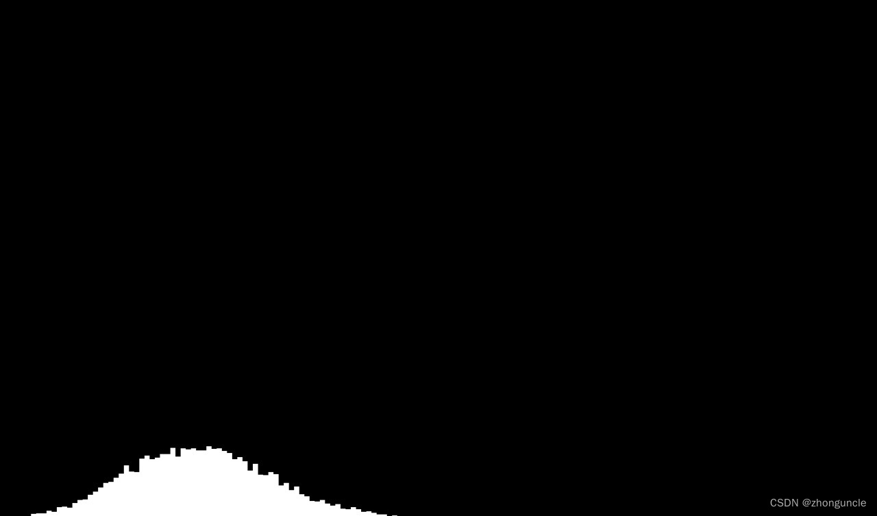
Now the image gengerated like:

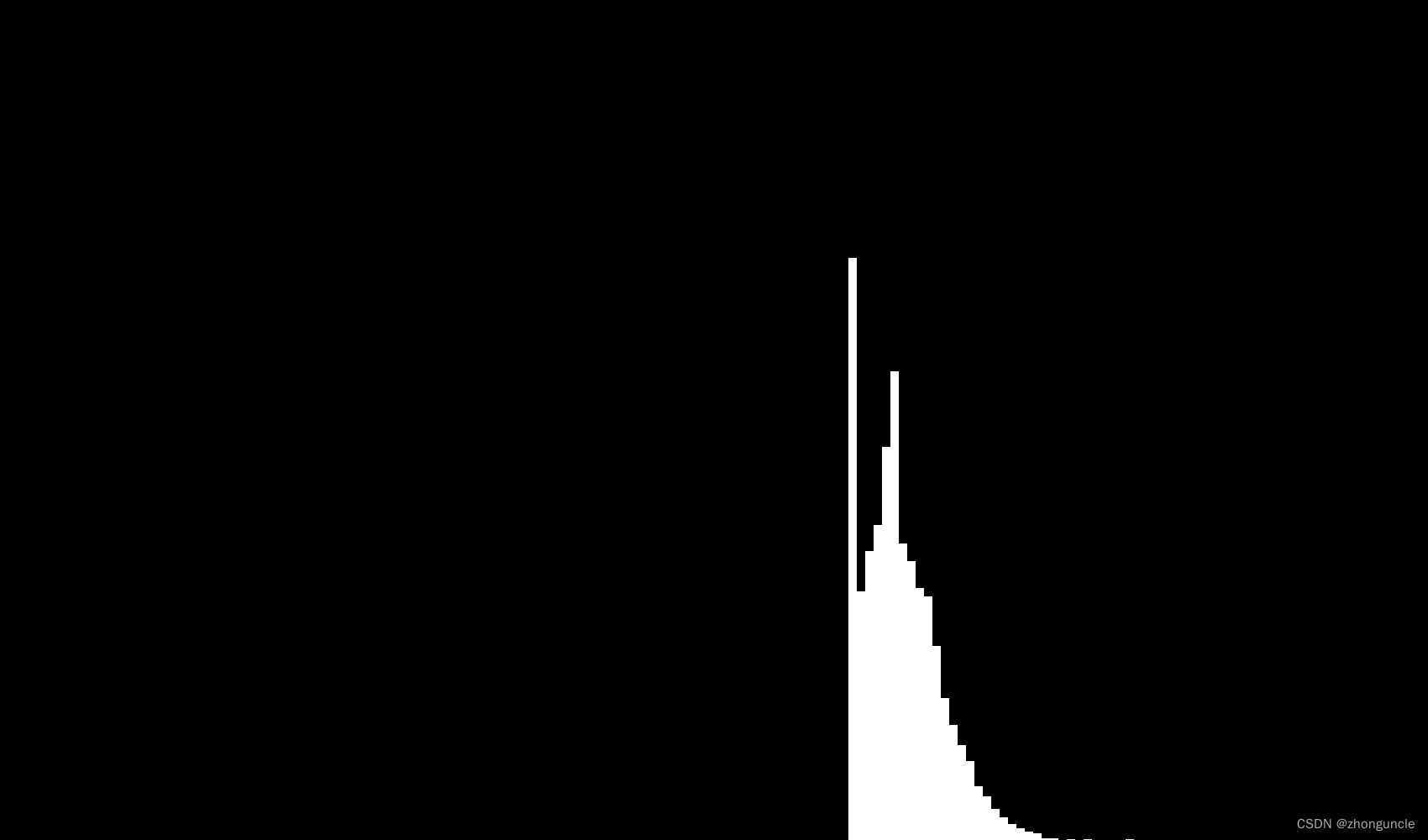
You can see the samples with the minimum value of ‘1+1=2’ are the most, but the right part still look like half of the normal distribution curve. What if increase the number of iterations? For example, from 100 to 1000 and the number of samples is reduced to 10000, the image at this time is as follows:

Due to too many possible results, the image size here is 17000x1000px, which is a bit unclear to see, so I have cropped out a part of the image:

Finally it still conforms to the normal distribution curve, which is also the central limit theorem.

It’s quite interesting. I hope these will help someone in need~