How LLMs Learn "Relationships": A word2vec Deep Dive
Translated by Claude Sonnet 5 (medium).
The core idea behind how today’s LLMs learn “relationships” from data traces all the way back to the classic word2vec.
Co-occurrence Matrix
Using a cleaned corpus, we can predict the next word just by counting the probabilistic relationship between a word and its neighbors. Here’s the classic example from CS224N:
The CS224N instructor is, in fact, one of the authors of GloVe.
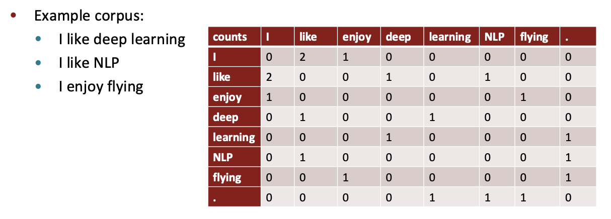
Suppose our corpus contains only these three sentences:
- I like deep learning.
- I like NLP.
- I enjoy flying.
After deduplication, there are only 8 tokens (including the period .):
{I, like, enjoy, deep, learning, NLP, flying, .}
Assume a window size of 1 (i.e. we only look at the 1 neighboring word on each side):
- After I: “like” appears 2 times, “enjoy” appears 1 time, 3 total. So the next word is “like” with 66.7% probability, “enjoy” with 33.3%;
- After like: “deep” appears 1 time, “NLP” appears 1 time, 2 total. So “deep” and “NLP” are each 50% likely to come next;
- After enjoy: “flying” appears 1 time out of 1 — 100% probability;
- After deep: “learning” appears 1 time out of 1 — 100% probability;
- After learning: the period “.” appears 1 time out of 1 — 100% probability;
- After NLP: same — the period follows with 100% probability;
- After flying: same — the period follows with 100% probability.
This is essentially the core algorithm behind predictive text input, also known as a Markov chain. Claude Academy has an interactive tutorial that makes this a lot more intuitive: Texting a Friend: The Markov Chain Edition – Claude Academy.
But this is nowhere near enough to get to today’s LLMs:
-
LLMs use a much larger window (they can read everything that came before, not just one neighboring word);
Worth noting: LLMs are decoder-only — they can only read what came before, never what comes after.
You might wonder what “reading what comes after” even means. Everything derived from the Transformer really only does two kinds of work: continuation and fill-in-the-blank. Fill-in-the-blank requires looking at both sides of the context, not just what came before.
An encoder can read in both directions; a decoder can only read what precedes it. I’ll dig into this in a separate post.
-
LLMs use far more sophisticated machinery to fit far more complex patterns (billions of parameters, attention, embeddings, residual connections, and so on — not just a simple lookup table).
But at their core, both are doing the same thing: predicting the next word (or token, really).
You might think this example feels out of place — like it has nothing to do with embeddings or modern LLMs. So what’s the point?
An embedding turns a sentence or a word into a vector representation so we can compute similarity between them. But look — if you drop the word itself from each row of that co-occurrence table, isn’t each remaining row already a vector?
Take the rows for “like” and “enjoy”:
| Word | Vector |
|---|---|
| like | [2, 0, 0, 1, 0, 1, 0, 0] |
| enjoy | [1, 0, 0, 0, 0, 0, 1, 0] |
The cosine similarity between these two vectors is about 0.5774. That’s not especially meaningful here, though, since our corpus is only three sentences — there’s not much to learn from. We can apply SVD to reduce dimensionality (notice most entries in these vectors are 0, and once you stack them into a matrix, most of the matrix is 0 too — so it compresses nicely into a smaller one). Here we reduce down to 2 dimensions (note: at this point there’s no longer a single number that directly represents “the relationship between word A and word B”):
| Word | Dim 1 | Dim 2 |
|---|---|---|
| I | -1.445 | -1.534 |
| like | -1.639 | 1.688 |
| enjoy | -0.707 | 0.734 |
| deep | -0.788 | -0.664 |
| learning | -0.533 | 0.091 |
| NLP | -0.841 | -0.787 |
| flying | -0.503 | -0.431 |
| . | -0.681 | 0.421 |
Since we’re in 2D, plain Euclidean distance (the everyday distance formula) works fine. Pairwise distances:
| I | like | enjoy | deep | learning | NLP | flying | . | |
|---|---|---|---|---|---|---|---|---|
| I | 0 | 3.228 | 2.385 | 1.091 | 1.864 | 0.960 | 1.450 | 2.100 |
| like | 3.228 | 0 | 1.334 | 2.501 | 1.943 | 2.600 | 2.404 | 1.588 |
| enjoy | 2.385 | 1.334 | 0 | 1.400 | 0.666 | 1.527 | 1.183 | 0.314 |
| deep | 1.091 | 2.501 | 1.400 | 0 | 0.797 | 0.135 | 0.367 | 1.090 |
| learning | 1.864 | 1.943 | 0.666 | 0.797 | 0 | 0.931 | 0.523 | 0.362 |
| NLP | 0.960 | 2.600 | 1.527 | 0.135 | 0.931 | 0 | 0.491 | 1.219 |
| flying | 1.450 | 2.404 | 1.183 | 0.367 | 0.523 | 0.491 | 0 | 0.871 |
| . | 2.100 | 1.588 | 0.314 | 1.090 | 0.362 | 1.219 | 0.871 | 0 |
Smaller values here mean the words are closer in meaning.
For example, “like” and “enjoy” are both verbs, so they end up somewhat close together. But you can also find counterexamples — “enjoy” and “learning” end up even closer, even though one is a verb and the other a gerund. That’s simply because they happen to co-occur a lot in this tiny corpus.
So it comes back to the same issue: the corpus is too small, and distances in 2D are inherently unstable. Take this as a rough intuition — the real point is understanding how text gets turned into vectors in the first place (counting neighboring-word frequency is just one approach; the underlying logic is always representing a word with some kind of vector).
This is actually a broader issue in model training in general: the corpus needs to be both high-quality and large. Data cleaning today is quite advanced — some of it is even automated by other models — but in the early days, corpus quality had an outsized effect on model performance.
In CS224N, GloVe co-author Chris Manning mentions that at the time, they were thrilled their model clearly outperformed word2vec and assumed their design was simply better. Years later, they realized the improvement was probably mostly due to a better training corpus, not the architecture. Timestamp 52:43 in Stanford CS224N NLP with Deep Learning | Winter 2021 | Lecture 2 - Neural Classifiers.
One more thing — Markov chains are a great way to feel the magic of probability. Probability is the foundation of large language models, and one of the foundations of information theory too. I can’t think of many other examples that let you see, this intuitively, how probability theory pulls off the marvel that is an LLM. You really do need to build an intuition for how powerful probability theory is.
And while a lot of people will tell you embeddings are “just vectors” (i.e. linear algebra), how they actually end up distributed — and which outcome gets chosen — is fundamentally a probability question.
LLMs are one of humanity’s great achievements. They’re digital, but they’re the first time human intelligence and reasoning have been externalized — the same way machines externalized physical strength, letting us scale it far beyond what any human body could ever do on its own.
But underneath it all, it’s just probability. In the public imagination, probability has always been tangled up with gambling, fortune-telling, and mysticism — even textbooks mostly illustrate it with dice and playing cards. It’s hard to look at that and realize probability theory is capable of pulling off a wonder like this (though I suppose Las Vegas counts too).
Embeddings
Now let’s talk about how embeddings actually make “relationships” emerge.
The most direct way to see relationships emerge is to train an embedding model from scratch. I won’t dump a lot of code here — the point is the underlying idea, not the implementation. (Once you understand the idea, you can just have an AI write the implementation for you.)
For this experiment I used the first 20MB of the Text8 dataset (running the full thing on a MacBook Air M5 would take a while). Note: the project’s actual full training run used the first 60MB; the stats in this section and the A/B experiments below are all from the 20MB subset.
Text8 is Matt Mahoney’s cleaned version of the March 2006 English Wikipedia dump (tags/punctuation stripped, lowercased, whitespace-tokenized — great for research). The first 20MB has 3,416,066 raw tokens; after dropping words with frequency below 5 (min_count=5), 3,299,364 tokens remain, with a vocabulary of 29,428 words.
Preprocessing
First we need to preprocess the dataset a bit (even though it’s already well-cleaned, training still needs a bit more prep).
Subsampling
First we need to remove some high-frequency words (like “the”, “of”, “and”), because they eat up training iterations that could otherwise go to low-frequency words.
Subsampling is the standard way to handle high-frequency words — probabilistically dropping some of them. Rather than a fixed ratio, each word’s retention probability depends on its frequency:
\[P(\text{keep}) = \sqrt{t / f} \qquad t = 10^{-4} \text{ (threshold)},\ f = \text{the word's frequency}\]The higher a word’s frequency, the lower its retention probability. For example, “the” ends up with a retention rate of only about 4% (out of every 100 occurrences, roughly 4 are randomly kept), while a mid-frequency word like “king” is almost always kept.
In my run:
| Metric | Count |
|---|---|
| Total tokens (after dropping low-freq words) | 3,299,364 |
| Retained after subsampling | 1,614,418 |
| High-frequency tokens dropped | 1,684,946 (51.1%) |
You can see just how dominant these high-frequency words are — over half the tokens. That means most of the word pairs generated would involve high-frequency words, and most of the training budget was going toward that. Removing them either doubles the effective number of training iterations in the same amount of time, or halves total training time.
Experiment: high-frequency words don’t fatally distort the distribution
Since “the” — the highest-frequency word in English — is so often followed by a noun, my initial guess was that if we kept high-frequency words, training might end up clustering nearly every noun around “the,” making it hard to distinguish relationships between the nouns themselves. In other words, I initially assumed these high-frequency words would distort the relationships between other words.
The original paper has a footnote making a related point: syntactic patterns are a notable exception here — verbs strongly avoid following determiners, and past-tense verbs strongly avoid following “be” verbs or modals.
So I had an AI write a quick test comparing the with-subsampling and without-subsampling cases. The result was surprising — barely any difference:
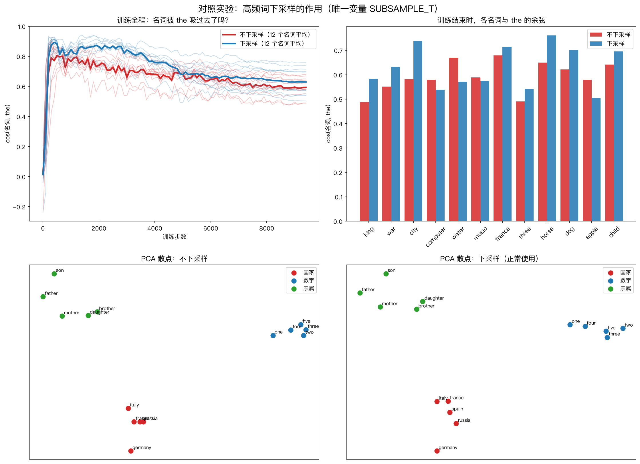
The result was the opposite of what I predicted:
- Similarity scores with subsampling were actually higher than without it (true both mid-training and at the end).
- The distributions with and without subsampling look pretty similar (though subsampling gives slightly better results — no words end up crammed unnaturally close together).
So what’s the actual point of subsampling, then?
-
It’s faster. In this run, subsampling removed 51% of the filler tokens and still gave slightly better results — meaning roughly half the training time saved.
-
The effective sliding window gets bigger. Some words that used to be “blocked” from pairing up by a “the” sitting between them now get paired once “the” is removed. This effectively widens the sliding window without actually changing its size.
-
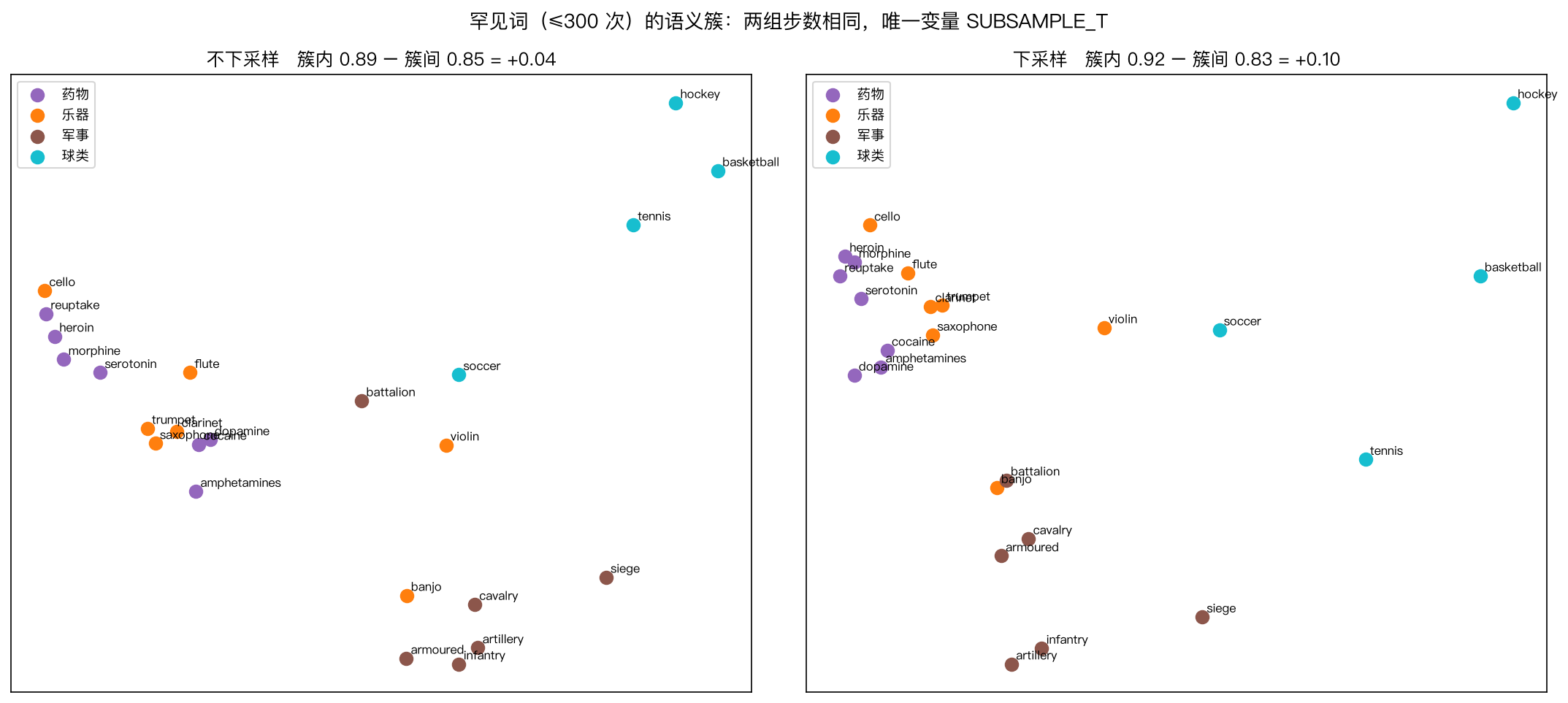
It improves low-frequency word representations. High-frequency words stop changing much after enough training samples, so continuing to train on them is wasted effort. Since the total training budget is fixed, that saved budget effectively goes to low-frequency words instead. You can see in the chart below that after subsampling, related word types cluster together noticeably better.
Sliding-window pairing
Following the original paper’s design: the sliding window has a radius of 5, and the further away a neighbor is, the lower its chance of being kept.
Here’s the process:
Input: a sequence of word IDs (post-subsampling, all sentences concatenated into one long text), with window radius window = 5.
Corpus: ... once in the land the king ruled his kingdom and the queen wore her crown ...
Each step centers the window on one word and looks up to 5 words in each direction (10 candidate neighbors total). But not all 10 get paired: each center word first randomly draws an “effective radius” $r$ (uniformly from 1 to 5), and only pairs with neighbors within distance $\le r$; anything farther gets skipped.
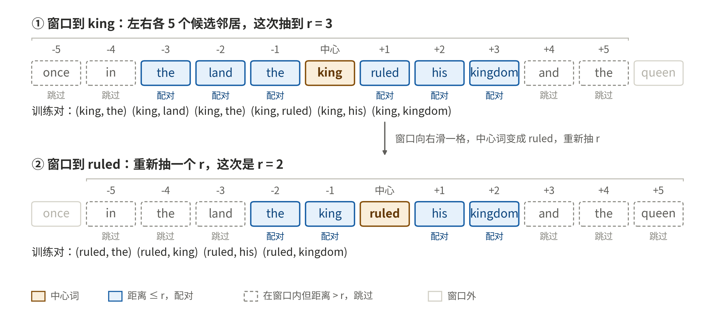
In the first step shown, the window centers on king, draws r = 3, and produces 6 pairs:
(king, the) (king, land) (king, the) (king, ruled) (king, his) (king, kingdom)
In the second step, the window slides one position right, centering on ruled, redraws r — this time getting r = 2 — and produces 4 pairs:
(ruled, the) (ruled, king) (ruled, his) (ruled, kingdom)
This keeps sliding one position at a time across the whole corpus. The value of r determines the number of pairs:
r = 1 → 2 pairs
r = 2 → 4 pairs
r = 3 → 6 pairs
r = 4 → 8 pairs
r = 5 → 10 pairs
The probability a neighbor at distance $d$ gets kept is $\dfrac{W - d + 1}{W}$ (which follows from drawing $r$ uniformly from 1 to $W$ — this matches the actual word2vec implementation). For $W = 5$:
distance 1 (adjacent):  100% kept
distance 3:              60% kept
distance 5 (farthest):   20% kept
So each center word ends up with somewhere between 2 and 10 pairs (always an even number), averaging 6. That means, after running the sliding window over the 1.61-million-token corpus (post-subsampling) in this experiment, we ended up with roughly 9.7 million training pairs.
From here on, training only uses these pairs — the original text file and extracted corpus are no longer needed.
That wraps up preprocessing. Next comes actual model training.
Training
After preprocessing, we ended up with about 9.7 million (center word, context word) pairs. Training only needs these pairs — the original corpus is no longer necessary, since we’ve already converted it into this pair structure.
W_in and W_out: the trained weight matrices
During training, every word gets two corresponding vectors — these are the parameters (weights) actually being trained in an embedding model.
One vector is used when the word plays the role of “center word” (W_in), the other when it plays the role of “context word” (W_out). After training, W_out is simply discarded, and W_in becomes the final set of word vectors. That’s what lets us see relationships between different words — specifically, the relationships between their “center-word” vectors.
This idea shows up all over the place, in computing and in human society alike.
In a database, for example, you can identify a record with a UUID, or you can identify it through its various attributes instead.
Or, as a person, you can be identified by an ID number, or by your web of relationships — whose child you are, whose partner, whose student or teacher, and so on.
So why bother with two separate vectors?
W_in is like your “ID number”; W_out is more like “relationships.”
Here’s an analogy. Imagine handing out ID numbers 1–100 to a group of people, assigned randomly — the numbers don’t encode rank or closeness, and once assigned they’re fixed forever. Looking at two people’s ID numbers in real life tells you nothing about their relationship.
But an embedding’s “ID number” is different: we get to keep nudging it before it’s finalized. If I discover two people are family, I move their numbers a bit closer together; if two people are coworkers, I nudge those closer too. After tens of millions of these tiny adjustments, the once-random numbers stop being random: numbers that end up close together tend to belong to people who are actually close.
That’s exactly what training is: W_in starts out as randomly assigned “numbers” (see the initialization below), and training is just the repeated process of nudging those numbers until the numbers themselves end up encoding relationships.
Parameters need to be initialized before training starts, and a good initialization leads to better results and faster convergence:
W_outis initialized to all zeros — at the start, the model scores every word pair as 0, meaning “totally unsure.” A neutral starting point.W_inis initialized with small random values in $-0.05$ to $0.05$. It can’t be all zeros (every word would be perfectly symmetric with identical gradients, so nothing would ever differentiate), but it also can’t be too small.
What happens if it’s too small?
config.pylogs one real measurement (30MB corpus, 3 epochs):
Init scale Dims needed for 90% variance Avg cosine (any two words) 0.005 (original word2vec) 17 0.385 0.05 (this project’s default) 47 0.320 0.1 67 0.301 When the init scale is too small, only a dozen or so of the 100 dimensions actually end up doing any work, badly hurting the vectors’ ability to distinguish words. Everything ends up crammed together, with cosine similarities clustering around 0.99.
This also interacts with corpus size — a large enough corpus and enough epochs can partly work around this. That’s why the original paper used 0.005, while our smaller corpus needed to bump it up to 0.05.
Negative sampling
Negative sampling means randomly drawing a handful of unrelated words to use as negative examples. Here we use $f^{0.75}$ negative sampling — sampling proportional to word frequency raised to the 0.75 power. Concrete example: suppose the vocabulary has just 3 words, in a 1-million-token corpus:
| Word | Count | Frequency $f$ | Uniform sampling ($f^0$) | Frequency-proportional ($f^1$) | $f^{0.75}$ |
|---|---|---|---|---|---|
| the | 60,000 | 0.06 | 33.3% | 98.5% | 96.3% |
| king | 600 | 0.0006 | 33.3% | 0.99% | 3.0% |
| zebra | 100 | 0.0001 | 33.3% | 0.16% | 0.8% |
How the $f^{0.75}$ column is computed: give each word a “weight” of $f^{0.75}$, then normalize.
- the: $0.06^{0.75} \approx 0.121$
- king: $0.0006^{0.75} \approx 0.00382$
- zebra: $0.0001^{0.75} = 0.001$
Summing to $\approx 0.1258$ and dividing each weight by that sum gives the sampling probabilities: the ≈ 96.3%, king ≈ 3.0%, zebra ≈ 0.8%.
Comparing the three columns shows what raising to the 0.75 power actually buys you:
- $f^1$ (raw frequency): “the” dominates at 98.5% — negative examples are almost always the/of/and, which the model can trivially push away without learning anything useful;
- $f^0$ (uniform): rare words like “zebra” get pulled 1/3 of the time, even though they have nothing to do with most center words — pushing them away is also too easy, so again nothing useful is learned;
- $f^{0.75}$: “the” is still the most-sampled word (96.3%), but low-frequency words get a meaningful boost — “zebra” jumps from 0.16% to 0.8% (5x), “king” from ~1% to 3%.
This “just a few negative words per step” approach is entirely a time-budget decision. You might wonder whether it’s too limited — after all, we could just use softmax and compare a word against the entire vocabulary every step, but that would make training dramatically slower. I ran a comparison experiment on exactly this later on, so you can see the difference for yourself.
How the weights actually get trained
As mentioned, each training pair is (center word, context word), plus 5 negative words drawn via negative sampling for that step. Call them center word $c$, context word $o$, and negative words $w_1 \dots w_5$. The training step:
\[\begin{aligned} \text{score} \quad & s = v_c \cdot u_x \\ \text{probability} \quad & \sigma(s) = \frac{1}{1 + e^{-s}} \\ \text{error} \quad & g = \sigma(s) - y \end{aligned}\]The score is just a dot product between two vectors — the more alike they are, the higher the score. Sigmoid squashes any score into 0–1, turning it into a confidence that “these two really are a pair.” $y = 1$ for a true context word, $y = 0$ for a negative word.
Training uses $g$ to decide whether to pull the two vectors closer together or push them apart. A negative $g$ pulls them together; a positive $g$ pushes them apart. The entire training process is just this one step repeated tens of millions of times.
For example, with 5 words [king, queen, the, banana, war] and the training pair (king, queen), suppose the dot products with king have already been computed, and the negative samples drawn happen to be “the” and “banana”:
| Question | $y$ | $s$ | $\sigma(s)$ | $g = \sigma(s) - y$ | Interpretation |
|---|---|---|---|---|---|
| Is queen a pair? | 1 | +2.0 | 0.881 | −0.119 | Already good — nudge slightly closer |
| Is “the” a pair? | 0 | +1.0 | 0.731 | +0.731 | Too similar — push hard apart |
| Is “banana” a pair? | 0 | 0.0 | 0.500 | +0.500 | No idea yet — push apart moderately |
“war” wasn’t drawn for this step, so its vector doesn’t get updated this round.
After tens of millions of interactions like this, the relative positions of “king” and “queen” settle down, and that’s when we start seeing the relationship between them emerge.
The
trace.pyscript in my embeddingTest project can print out one real training step exactly like this table (every intermediate value maps onto the formulas above) — the numbers you see are from actual training, not a toy example.
A few training-loop details
- Subsampling is redone every epoch: different high-frequency words get dropped each time, so each epoch effectively sees a slightly different corpus — a mild form of data augmentation.
- Learning rate decays linearly: from 0.025 down to near 0.
What does this look like in practice? Log from the actual training run (60MB, 2 epochs):
subsampling : 9,971,789 -> 5,019,569 tokens (50% of high-frequency tokens dropped)
pairs       : 30,119,260 pairs / epoch (60MB corpus; the 9.7M-pair figure earlier was from the 20MB experiment)
speed       : ~230k pairs/sec, 273 seconds total (Apple Silicon MacBook Air, pure numpy)
loss        : 3.69 -> 2.32
Worth sanity-checking against theory: pure guessing gives $\sigma = 0.5$, so the loss per comparison is $\ln 2 \approx 0.693$, or about 4.16 for 6 comparisons. Loss dropping from 3.69 to 2.32 confirms the model is genuinely learning something — though loss here is really just a byproduct; the real payoff lives in the vectors themselves.
Experiment: negative sampling vs. full softmax
If negative sampling is really just a compromise because “full softmax is too expensive,” what does that compromise actually cost you? I had an AI write a comparison script (compare.py): the same skip-gram model, only swapping out the output layer — one version uses negative sampling, the other does full-vocabulary softmax.
My original prediction: I figured the two would differ mainly in speed, with similar quality — after all, “sample enough times and everything gets its turn eventually.”
I was only half right. With a small vocabulary and a small corpus (3MB), negative sampling completely fell apart: no matter how I tuned the learning rate, batch size, or step count, the word vectors collapsed into a clump — cosine similarity between any two random words hit 0.94, and nearest-neighbor results were pure noise. Softmax, meanwhile, worked fine on the exact same data. Scaling the corpus up to 30MB (vocabulary unchanged) fixed negative sampling immediately.
The mechanism, roughly:
- Softmax pushes everything, every time. Every step applies a repulsive force to every non-answer word in the vocabulary — no exceptions, no relying on luck. Take the same 5 scores from before (+2.0, +1.0, 0, −1.0, −2.0); softmax converts these into probabilities $P(\text{queen}) = 0.636$, $P(\text{the}) = 0.234$, $P(\text{banana}) = 0.086$, $P(\text{war}) = 0.032$, $P(\text{king}) = 0.012$, and each word gets pushed by “probability − target value”: queen gets pulled closer by 0.364, “the” gets pushed by 0.234, “war” by only 0.032 — the push is automatically proportional to how wrong the current prediction is;
- Negative sampling pushes only a sample, each time. Each step only pushes 5 unrelated words away — this sparse repulsion needs a large amount of non-repeating data before it averages out statistically. On a small corpus, words simply don’t “get their turn” often enough to be pushed apart properly, so everything collapses inward.
This also explains why negative sampling was designed with web-scale corpora in mind: only with enough data does the statistical average of “push a sample away” actually hold, and only then does the $O(V)$ compute it saves actually pay off.
One more interesting detail: the two setups can’t share a learning rate. Softmax’s gradient gets spread thin across the whole vocabulary — negative sampling’s 0.025 barely moves it. It needed 0.2 to train properly, and diverged at 1.0. Needing different learning rates is itself pretty direct evidence that these are two fundamentally different optimization problems.
Summary
The relationships between words emerge naturally from “learning” — they’re not designed in, the way you might explicitly teach a human reasoning or logic. We never told the model what any particular dimension should mean, or how to represent relationships, identity, and so on — all of that emerges purely from the training process.
By “learning” here, I mean the process of fitting a statistical/probabilistic model on a large amount of training data — not that the model is actually learning on its own in any deeper sense.
Extra: how do you compute sentence similarity?
The simplest approach: average the vectors of every word in a sentence to get a sentence vector (called mean pooling), then compare sentences pairwise with cosine similarity.
That’s exactly what demo.py in the project does — for example, these two sentences come out highly similar:
- the king ruled his kingdom
- the queen governed her empire
Because king/queen, ruled/governed, and kingdom/empire already sit close together in vector space, averaging naturally lands the two sentence vectors close together too.
But this approach has two obvious holes:
- It throws away word order. “I love you” and “you love I” use exactly the same words, so their averaged vectors are identical — similarity of 1 — even though the two sentences clearly mean different things (“dog bites man” vs. “man bites dog” has the same problem: one’s news, the other isn’t).
- Unknown words just get dropped. Any word not in the vocabulary is silently skipped, as if it didn’t exist.
Sentence-embedding models like BERT and SBERT exist mainly to solve exactly these two problems.
References
Texting a Friend: The Markov Chain Edition – Claude Academy — a nicely interactive resource that helps build intuition.