Introduction to Maximum Likelihood Estimation and How to Automatically Learn Parameters with Code (ML/DL)

2025-07-28 ｜ Research ｜ #Words: 4502 ｜中文原版

Maximum Likelihood Estimation (MLE): A Practical Guide with Code

Maximum Likelihood Estimation (MLE), also translated as “maximum likelihood estimation,” is a method for obtaining the optimal parameters of a model from sample data.

For example, MLE can estimate the parameters of a probability density function. Suppose a set of samples/datasets/statistics (potentially) follows a normal distribution—by finding the mean, variance, or standard deviation of the dataset, we can derive the probability density function that fits the data.

\[f(x) = \frac{1}{\sqrt{2\pi\sigma^2}} e^{-\frac{(x - \mu)^2}{2\sigma^2}}\]

Where:

$\mu$ = mean
$\sigma^2$ = variance
$x$ = value of the random variable

MLE Workflow

The workflow for maximum likelihood estimation is as follows:

Determine the probability model: For example, the normal distribution model.
Construct the likelihood function: This involves multiplying all probability density functions together.

Alternatively, we can convert it to a logarithmic function, which turns the product into a sum—this is more convenient in many cases. Additionally, for computers, addition is computationally cheaper than multiplication.
As a side note: While the function itself is continuous, the samples are discrete, so the probability density function behaves as “discrete” and can be multiplied sequentially.

Maximize the log-likelihood function

For each data point, we substitute the current $x$ into the function (e.g., the standard normal distribution function). The independent variables of the likelihood function are the model parameters. We then take the derivative to find the optimal solution for the MLE parameters.
For program implementation, the derivative tells us the direction of parameter adjustment.

Demonstrating How Machines Learn Parameters via MLE

You may have found this article while studying for an exam, but once you understand the principles of MLE, it largely boils down to memorizing formulas. So let’s instead demonstrate how to obtain estimated parameters through code.

We’ll start with arbitrary parameters for a normal distribution probability density function: $\mu = 7.2$ and $\sigma = 2.8$ (which means $\sigma^2 = 7.83999$).

We’ll begin with the standard normal distribution (you can start with others) and continuously adjust the parameters until they match our target parameters.

First, we’ll generate 100,000 data points using the target parameters as our sample. We’ll then fit the MLE parameters to this sample.

This differs from textbook problems in two ways: 1) We’re estimating two parameters instead of one, and 2) We’re not using derivatives to find the solution directly.

Below are key code snippets (with explanations in comments)—see the full code later:

def __init__(self):
    # Target distribution parameters
    self.target_mu = 7.2    # Theoretical mean
    self.target_sigma = 2.8 # Theoretical standard deviation
    self.target_var = self.target_sigma ** 2  # Theoretical variance
    
    # MLE estimated parameters
    self.mle_mu = 0.0       # Estimated mean
    self.mle_sigma = 1.0    # Estimated standard deviation
    self.mle_var = self.mle_sigma ** 2  # Estimated variance

Next, generate the data:

def generate_data(self, n_samples=100000):
    """Generate observed data"""
    self.data = np.random.normal(
        loc=self.target_mu,
        scale=self.target_sigma,
        size=n_samples
    )
    print(f"Generated {n_samples} data points from N(μ={self.target_mu}, σ²={self.target_var:.2f})")
    
    # Theoretical MLE values (sample statistics)
    # Note: Sample statistics differ slightly from theoretical values (shown later)
    self.true_mle_mu = np.mean(self.data)
    self.true_mle_var = np.var(self.data, ddof=0)
    self.true_mle_sigma = np.sqrt(self.true_mle_var)
            
    return self.data

Now perform maximum likelihood estimation:

def mle_gradient_descent(self, epochs=10000, lr=0.05, tol=1e-8):
    # Manually split into training and validation sets (no separate test set)
    # This is a common technique
    train_data, val_data = train_test_split(self.data, test_size=0.2, random_state=42)
    
    # Initialize parameters
    self.mle_mu = self.initial_mu
    self.mle_var = self.initial_var
    self.mle_sigma = np.sqrt(self.mle_var)
    
    # For logging and plotting
    self.train_log_likelihoods = []
    self.val_log_likelihoods = []
    self.epochs_record = []
    best_val_ll = -np.inf
    best_mu, best_var = self.mle_mu, self.mle_var
    
    # For early stopping to prevent overfitting
    counter = 0 
    
    # Start training
    for epoch in range(epochs):
        # Convert to log-likelihood for easier computation
        # loc=self.mle_mu: location parameter (mean)
        # scale=np.sqrt(self.mle_var): scale parameter (standard deviation)
        # Log transformation converts product to sum, reducing computational cost
        # Note: Closer to 0 indicates better fit to training data
        train_ll = np.sum(stats.norm.logpdf(train_data, loc=self.mle_mu, scale=np.sqrt(self.mle_var)))
        val_ll = np.sum(stats.norm.logpdf(val_data, loc=self.mle_mu, scale=np.sqrt(self.mle_var)))
        
        # Log values for plotting
        self.train_log_likelihoods.append(train_ll)
        self.val_log_likelihoods.append(val_ll)
        self.epochs_record.append(epoch + 1)
        
        # Calculate errors
        error = train_data - self.mle_mu 
        # Gradient of the mean
        grad_mu = np.mean(error / self.mle_var)
        # Mean squared error between training data and estimated variance
        mean_squared_error = np.mean(error ** 2)
        # Gradient of the variance
        grad_var = (-1/(2*self.mle_var)) + (mean_squared_error)/(2*self.mle_var ** 2)
        
        # Update parameters (gradient ascent)
        self.mle_mu += lr * grad_mu
        self.mle_var += lr * grad_var
        # Ensure variance is non-negative
        self.mle_var = max(self.mle_var, 0) 
        # Update standard deviation (for early stopping)
        # We initially designed with standard deviation, not variance
        self.mle_sigma = np.sqrt(self.mle_var)
        
        # Early stopping: stop if validation log-likelihood doesn't improve for 50 epochs
        if val_ll > best_val_ll:
            best_val_ll = val_ll
            best_mu, best_var = self.mle_mu, self.mle_var
            counter = 0
        else:
            counter += 1
            if counter >= 50 or (abs(val_ll - best_val_ll) < tol):
                print(f"\nConverged at epoch {epoch+1}")
                self.mle_mu, self.mle_var = best_mu, best_var
                self.mle_sigma = np.sqrt(self.mle_var)
                break
        
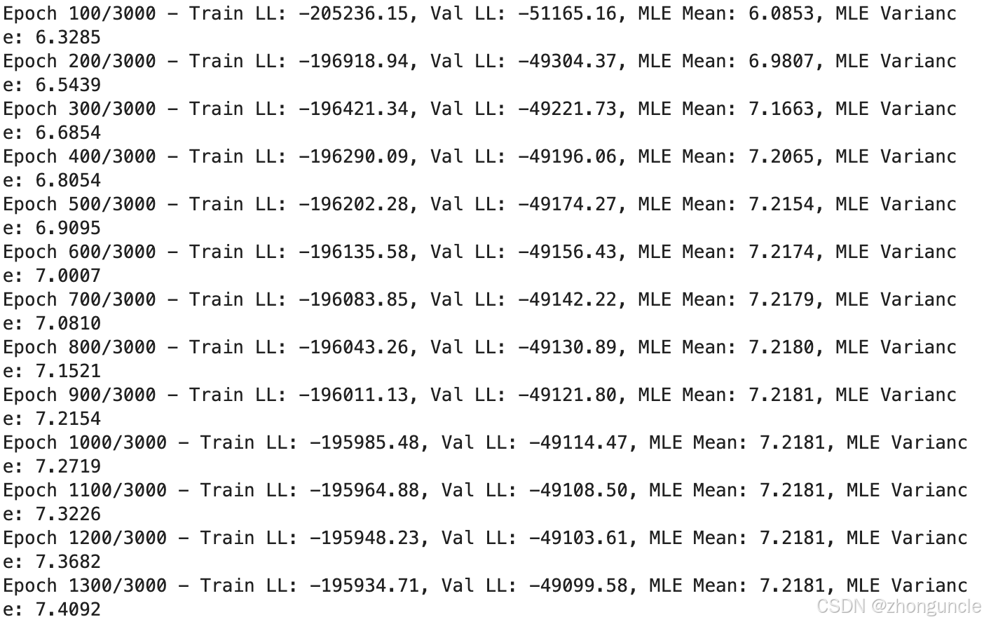
        # Print progress every 100 epochs
        if (epoch + 1) % 100 == 0:
            print(f"Epoch {epoch+1}/{epochs} - "
                  f"Train LL: {train_ll:.2f}, Val LL: {val_ll:.2f}, "
                  f"MLE Mean: {self.mle_mu:.4f}, MLE Variance: {self.mle_var:.4f}")
    
    return self.train_log_likelihoods

Let’s explain this critical code section:

# Calculate gradient of the mean
grad_mu = np.mean(error / self.mle_var)
# Mean squared error between training data and estimated variance
mean_squared_error = np.mean(error ** 2)
# Calculate gradient of the variance
grad_var = (-1/(2*self.mle_var)) + (mean_squared_error)/(2*self.mle_var ** 2)

In computer science, gradients and derivatives are often implemented using their basic definition: the rate of change. Unlike pure mathematics, real-world implementations don’t require complex limit calculations (as you can see from the code). However, we still need to compute the derivative for the variance gradient manually.

First, the log-likelihood function is: $\log L(\mu, \sigma^2) = -\frac{n}{2}\log(2\pi) - \frac{n}{2}\log(\sigma^2) - \frac{1}{2\sigma^2}\sum_{i=1}^n (x_i - \mu)^2$

Take the partial derivative with respect to $\sigma^2$ (note: $\sigma^2$, not $\sigma$): $\frac{\partial \log L}{\partial \sigma^2} = -\frac{n}{2\sigma^2} + \frac{1}{2\sigma^4}\sum_{i=1}^n (x_i - \mu)^2$

Factor out $\frac{n}{2\sigma^2}$: $\frac{\partial \log L}{\partial \sigma^2} = \frac{n}{2\sigma^2} \left( \frac{\sum (x_i - \mu)^2}{n\sigma^2} - 1 \right)$

The $n$ term (sample size) doesn’t affect the direction of parameter adjustment (it’s just a constant factor), so we can simplify it for computational efficiency: $\frac{\partial \log L}{\partial \sigma^2} = \frac{1}{2\sigma^2} \left( \frac{\sum (x_i - \mu)^2}{n\sigma^2} - 1 \right)$

While $\mu$ represents the mathematical expectation (mean) in theory, we use the estimated mean from the sample in practice.

An important note: The learning rate must be consistent for both parameters. As you’ll see in the training results, the mean converges much faster than the variance (due to the squared term in the variance calculation). Using different learning rates for each parameter will result in significant estimation errors.
Don’t just take my word for it—try experimenting with different learning rates and see for yourself.
Is there a solution? Yes—modern models often use adaptive learning rates (e.g., decreasing the learning rate when the loss plateaus to improve accuracy) or learning rate scheduling functions. However, this is beyond the scope of this blog and won’t be covered here.

Now let’s start training. Below is the full code—feel free to copy and run it yourself:

import numpy as np
import pandas as pd
import matplotlib.pyplot as plt
from scipy import stats
from sklearn.model_selection import train_test_split
import os
import time 

np.random.seed(42)

class MLENormalEstimator:
    def __init__(self):
        self.target_mu = 7.2 
        self.target_sigma = 2.8 
        self.target_var = self.target_sigma ** 2 
        
        self.initial_mu = 0.0
        self.initial_sigma = 1.0
        self.initial_var = self.initial_sigma ** 2
        
        self.mle_mu = self.initial_mu
        self.mle_sigma = self.initial_sigma
        self.mle_var = self.initial_var
        
    def generate_data(self, n_samples=100000):
        self.data = np.random.normal(
            loc=self.target_mu,
            scale=self.target_sigma,
            size=n_samples
        )
        print(f"Generated {n_samples} data points from N(μ={self.target_mu}, σ²={self.target_var:.2f})")
        
        self.true_mle_mu = np.mean(self.data)
        self.true_mle_var = np.var(self.data, ddof=0) 
        self.true_mle_sigma = np.sqrt(self.true_mle_var)
        
        return self.data
    
    def mle_gradient_descent(self, epochs=10000, lr=0.05, tol=1e-8):
        train_data, val_data = train_test_split(self.data, test_size=0.2, random_state=42)
        
        self.mle_mu = self.initial_mu
        self.mle_var = self.initial_var
        self.mle_sigma = np.sqrt(self.mle_var)
        
        self.train_log_likelihoods = []
        self.val_log_likelihoods = []
        self.epochs_record = []
        best_val_ll = -np.inf
        best_mu, best_var = self.mle_mu, self.mle_var
        counter = 0
        
        start_time = time.time()
        
        for epoch in range(epochs):
            train_ll = np.sum(stats.norm.logpdf(train_data, loc=self.mle_mu, scale=np.sqrt(self.mle_var)))
            val_ll = np.sum(stats.norm.logpdf(val_data, loc=self.mle_mu, scale=np.sqrt(self.mle_var)))
            
            self.train_log_likelihoods.append(train_ll)
            self.val_log_likelihoods.append(val_ll)
            self.epochs_record.append(epoch + 1)
            
            error = train_data - self.mle_mu
            grad_mu = np.mean(error / self.mle_var)
            mean_squared_error = np.mean(error ** 2)
            grad_var = (-1/(2*self.mle_var)) + (mean_squared_error)/(2*self.mle_var ** 2)
            
            self.mle_mu += lr * grad_mu
            self.mle_var += lr * grad_var
            self.mle_var = max(self.mle_var, 0)
            self.mle_sigma = np.sqrt(self.mle_var)
            
            if val_ll > best_val_ll:
                best_val_ll = val_ll
                best_mu, best_var = self.mle_mu, self.mle_var
                counter = 0
            else:
                counter += 1
                if counter >= 50 or (abs(val_ll - best_val_ll) < tol):
                    print(f"\nConverged at epoch {epoch+1}")
                    self.mle_mu, self.mle_var = best_mu, best_var
                    self.mle_sigma = np.sqrt(self.mle_var)
                    break
            
            if (epoch + 1) % 100 == 0:
                print(f"Epoch {epoch+1}/{epochs} - "
                      f"Train LL: {train_ll:.2f}, Val LL: {val_ll:.2f}, "
                      f"MLE Mean: {self.mle_mu:.4f}, MLE Variance: {self.mle_var:.4f}")
        
        end_time = time.time()
        self.train_duration = end_time - start_time 
        
        return self.train_log_likelihoods
    
    def evaluate(self):
        print("\n" + "="*80)
        print("                  MAXIMUM LIKELIHOOD ESTIMATION RESULTS")
        print("="*80)
        print(f"1. Training Duration: {self.train_duration:.4f} seconds") 
        print(f"\n2. Target Distribution:")
        print(f"   - Mean: {self.target_mu:.6f}")
        print(f"   - Variance: {self.target_var:.6f}")
        
        print(f"\n3. Theoretical MLE (Sample Statistics):")
        print(f"   - Mean MLE: {self.true_mle_mu:.6f}")
        print(f"   - Variance MLE: {self.true_mle_var:.6f}")
        
        print(f"\n4. Estimated MLE:")
        print(f"   - Estimated Mean: {self.mle_mu:.6f}")
        print(f"   - Estimated Variance: {self.mle_var:.6f}")
        
        print(f"\n5. Initial Parameters:")
        print(f"   - Initial Mean: {self.initial_mu:.6f}")
        print(f"   - Initial Variance: {self.initial_var:.6f}")
        
        print(f"\n6. Estimation Errors:")
        print(f"   - Mean Error: {abs(self.true_mle_mu - self.mle_mu):.8f}")
        print(f"   - Variance Error: {abs(self.true_mle_var - self.mle_var):.8f}")
        print("="*80 + "\n")
        
        # Plot log-likelihood curve
        plt.figure(figsize=(6, 4))
        plt.plot(self.epochs_record, self.train_log_likelihoods, label='Training Log-Likelihood', 
                 color='blue', linewidth=1.2)
        plt.plot(self.epochs_record, self.val_log_likelihoods, label='Validation Log-Likelihood', 
                 color='orange', linewidth=1.2)
        plt.title('Log-Likelihood During MLE Optimization', fontsize=10)
        plt.xlabel('Epoch', fontsize=8)
        plt.ylabel('Log-Likelihood (Higher = Better)', fontsize=8)
        plt.grid(True, linestyle='--', alpha=0.5)
        plt.legend(fontsize=7)
        plt.tight_layout()
        plt.savefig('corrected_mle_log_likelihood.png', dpi=150)
        plt.close()
        
        # Plot distribution comparison
        plt.figure(figsize=(6, 4))
        x_min = min(self.data.min(), self.target_mu - 4*self.target_sigma, self.initial_mu - 4*self.initial_sigma)
        x_max = max(self.data.max(), self.target_mu + 4*self.target_sigma, self.initial_mu + 4*self.initial_sigma)
        x = np.linspace(x_min, x_max, 1000)
        
        plt.hist(self.data, bins=100, density=True, alpha=0.6, color='blue',
                 label=f'Observed Data (μ={self.true_mle_mu:.2f})')
        plt.plot(x, stats.norm.pdf(x, self.target_mu, self.target_sigma), 'g-', lw=2,
                 label=f'Target Distribution')
        plt.plot(x, stats.norm.pdf(x, self.mle_mu, self.mle_sigma), 'r--', lw=2,
                 label=f'Estimated MLE Distribution')
        plt.plot(x, stats.norm.pdf(x, self.initial_mu, self.initial_sigma), 'purple', ls=':', lw=1.5,
                 label=f'Initial Distribution')
        
        plt.title('Distribution Comparison', fontsize=10)
        plt.xlabel('Value', fontsize=8)
        plt.ylabel('Probability Density', fontsize=8)
        plt.legend(fontsize=7)
        plt.grid(alpha=0.3)
        plt.savefig('mle_distribution_comparison.png', dpi=150)
        plt.close()
        
        print("Generated plots:")
        print("1. corrected_mle_log_likelihood.png - Log-likelihood curve")
        print("2. mle_distribution_comparison.png - Distribution comparison (with initial curve)")

if __name__ == "__main__":
    estimator = MLENormalEstimator()
    estimator.generate_data(n_samples=100000)
    
    print("\nStarting maximum likelihood estimation...")
    estimator.mle_gradient_descent(
        epochs=10000,
        lr=0.1,
        tol=1e-8
    )
    
    estimator.evaluate()    

Sample Output (Truncated)

Epoch 9600/10000 - Train LL: -195870.32, Val LL: -49077.16, MLE Mean: 7.2181, MLE Variance: 7.8367
Epoch 9700/10000 - Train LL: -195870.32, Val LL: -49077.16, MLE Mean: 7.2181, MLE Variance: 7.8368
Epoch 9800/10000 - Train LL: -195870.32, Val LL: -49077.16, MLE Mean: 7.2181, MLE Variance: 7.8368
Epoch 9900/10000 - Train LL: -195870.32, Val LL: -49077.16, MLE Mean: 7.2181, MLE Variance: 7.8368
Epoch 10000/10000 - Train LL: -195870.32, Val LL: -49077.16, MLE Mean: 7.2181, MLE Variance: 7.8369

================================================================================
                  MAXIMUM LIKELIHOOD ESTIMATION RESULTS
================================================================================
1. Training Duration: 27.8044 seconds

2. Target Distribution:
   - Mean: 7.200000
   - Variance: 7.840000

3. Theoretical MLE (Sample Statistics):
   - Mean MLE: 7.202707
   - Variance MLE: 7.854133

4. Estimated MLE:
   - Estimated Mean: 7.218075
   - Estimated Variance: 7.836873

5. Initial Parameters:
   - Initial Mean: 0.000000
   - Initial Variance: 1.000000

6. Estimation Errors:
   - Mean Error: 0.01536817
   - Variance Error: 0.01726031
================================================================================

Generated plots:
1. corrected_mle_log_likelihood.png - Log-likelihood curve
2. mle_distribution_comparison.png - Distribution comparison (with initial curve)

As you can see, the “Estimated MLE” values are very close to both the “Theoretical MLE (Sample Statistics)” and the “Target Distribution”—and this only took 27 seconds.

If you’re willing to sacrifice some precision for speed, you can reduce the number of epochs. The mean (MLE Mean) stabilizes after around 1,000 epochs—most of the remaining training time is spent optimizing the variance (MLE Variance):

Log-likelihood curve showing early stabilization of mean estimation

The code generates visualization plots to intuitively compare the results:

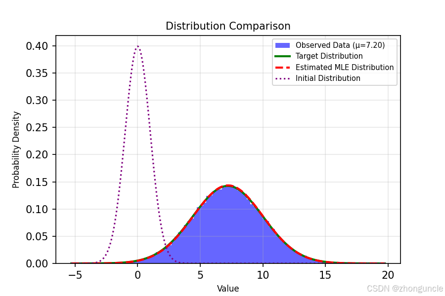
Distribution comparison: observed data, target distribution, estimated MLE distribution, and initial standard normal distribution

The purple dotted line on the left is the initial standard normal distribution.
The blue histogram is the sampled dataset.
The green solid line is the target distribution.
The red dashed line (appearing slightly orange here) is our estimated MLE distribution—you can see it’s nearly identical can see it’s nearly identical to the target.

A quick side note:
Even without any performance optimizations in Python, we achieved this level of precision in just 27 seconds. You might be thinking, “I can compute derivatives super fast—this seems pointless.”
But with C++ and optimizations (compiled with -O3), this takes only 1.6 seconds. If you adjust the random seed, early stopping might trigger after just 2-3 thousand epochs, reducing the time to 0.4 seconds.
And we haven’t even used SIMD parallel computing—with SIMD, the speed could be improved by several orders of magnitude.
Machine learning essentially learns parameters this way. Here, we only had 2 parameters to estimate—manageable even with manual calculations (and potentially more accurate). But modern large language models require describing relationships far more complex than normal distributions, leading to parameter counts in the billions. For example, DeepSeek’s largest model has 67.1B parameters (67.1 billion). This is humanly impossible to compute manually—let alone the increased computational complexity from advanced training architectures.
If you study the history of mathematics, you’ll find that beyond groundbreaking theorems, a significant amount of work focused on simplifying calculations. For example, logarithms were invented to simplify multiplication, and $e$ emerged to optimize logarithm tables.
Unfortunately, computational theory isn’t widely taught in China, so many people only learn about estimation methods and fitting techniques through specialized courses.
Early mathematicians didn’t just develop theories—they also built computing machines (Leibniz, for example, constructed his own calculator). We live in an era of unprecedented computational power, giving us tools previous generations could only dream of. Learning these estimation methods is therefore essential—even if they don’t seem “elegant” or “advanced” to some.

I hope these will help someone in need~