Encoder-Decoder vs. Encoder-only vs. Decoder-only: Comparing the Three Transformer Architectures
Translated by Claude Sonnet 5 (medium).
Three Transformer Architectures
The Full Transformer Architecture
The paper “Attention Is All You Need” introduced the Transformer architecture, built from an encoder and a decoder.
Architecture during training
Here’s what the Transformer looks like during training:
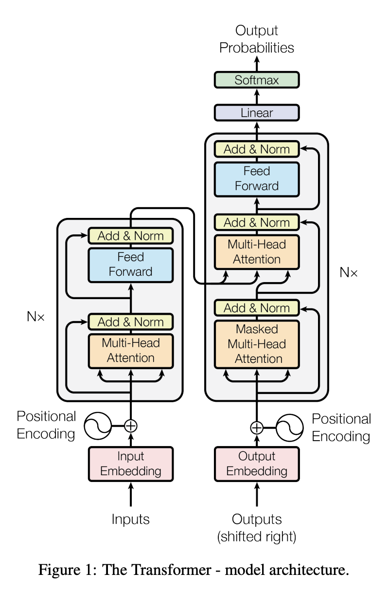
The left side is the encoder, the right side the decoder. The decoder has one extra piece — a masked multi-head attention block — everything else matches. That masked attention block is exactly what limits the decoder to only seeing tokens before the one it’s predicting, whereas the encoder can see everything.
This is actually the core difference between encoder and decoder — and it’s exactly what separates encoder-only from decoder-only models too.
At this point we’ve already answered the core question of this post, but what does that difference actually mean in practice?
Say we’re training a translation model, and we already have paired training data:
Inputs (to Encoder):  我 爱 北京
Outputs (to Decoder): I love Beijing   ← this is the "ground truth," already present in the training set
The training goal is for the decoder to learn: seeing <BOS> I love, predict Beijing. So that the decoder always has an “already generated prefix” to work with at every step, training just feeds it the ground-truth answer directly as if it were “already generated” — that’s exactly where the “Output Embedding” input comes from. It isn’t something the model generated itself; it’s the ground-truth answer from the training data, fed to the decoder as input.
Why “shift right”?
When the decoder predicts the $i$-th word, it should only be able to see words $1$ through $i-1$ (it must not see the very word it’s supposed to predict — that would be cheating). So the entire ground-truth sequence gets shifted one position to the right, with a <BOS> (Begin Of Sequence) token prepended:
Ground truth (Outputs):            I    love   Beijing
                                     ↓
Decoder's actual input (shifted): <BOS>  I     love
Decoder should predict at each:     I    love   Beijing
In other words, the decoder’s input at position $k$ is “the answer’s $(k-1)$-th word,” and it needs to predict “the answer’s $k$-th word.” Combined with masked multi-head attention (also called causal masking), this guarantees that predicting the $i$-th word only ever uses information from words $1$ through $i-1$ — no peeking at the future whatsoever. That’s how the model gradually learns the ability to predict the next word.
There’s a bit of a GAN-like feel to this — it’s called teacher forcing: the “teacher” (ground truth) holds the “student’s” (model’s) hand the whole way, so the student’s own mistakes never get a chance to compound.
In the training example above, the
<BOS> I love“input” is sliced directly from the ground-truth training data. No matter how accurate the model’s own predictions are, the next step is always fed the “correct prefix.” So even if step 2 predictslikesinstead oflove, step 3 still gets the correctloveto predict from — the model’s own error never gets a chance to drag it off course.
During training, the loss at each position is computed and used to keep adjusting the fit. And because the ground truth is already fully known — there’s no actual sequential dependency at training time — losses for all positions can be computed in parallel, which is much faster than a traditional RNN (inference is a different story, as we’ll see).
Here’s what gets updated during training:
| Diagram block | What it is |
|---|---|
| Input/Output Embedding (pink) | A “vocab-size × d_model” lookup table — each word maps to a vector, and these vectors are themselves parameters that get updated during training |
| Multi-Head Attention / Masked Multi-Head Attention (orange) | Each attention head has its own $W_Q, W_K, W_V$ (projecting input into Query/Key/Value) plus a shared $W_O$ that merges the heads’ outputs — these matrices are the core trainable parameters |
| Feed Forward (blue) | Two fully-connected layers (up-project then down-project); the weight matrices and biases inside are parameters, and usually make up the bulk of the model’s total parameter count |
| Norm part of Add & Norm (yellow) | LayerNorm has two small learnable parameters (scale γ and shift β) — tiny in count, but still parameters |
| Linear (purple, at the very top) | The final matrix that maps the decoder’s output back into vocab-size dimensions, producing a score for every word |
These parts never get updated during training:
- Add (the “+” in the residual connection): just a plain vector addition, no parameters involved
- Positional encoding (if using the original sine/cosine scheme from the paper): computed with a fixed formula, not trained (though many later models, like BERT, turned positional encoding into learnable parameters too — it varies by model)
- Softmax: a fixed mathematical function, no parameters
Architecture during inference
Since the original paper describes a full encoder-decoder framework, inference uses the exact same framework (training and inference share the same architecture — otherwise the trained weights for whichever part got dropped would simply vanish, and missing a piece would hurt generation quality):
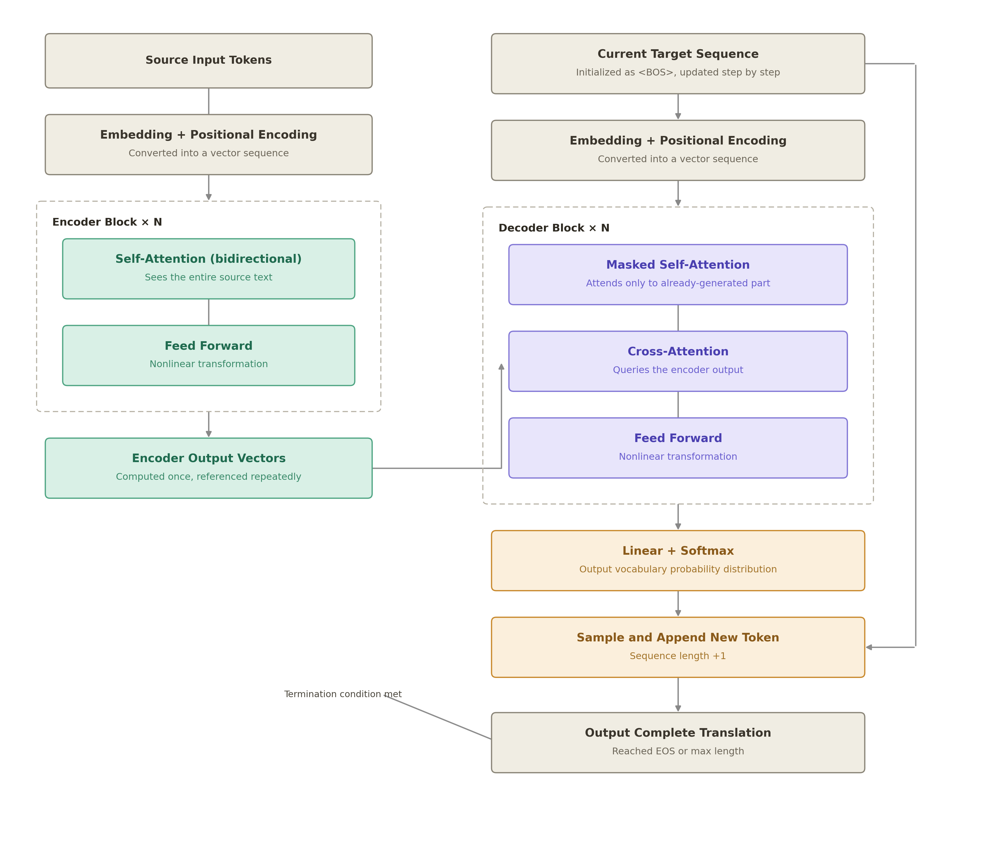
- The encoder on the left runs exactly once. The source text goes in, gets processed once with bidirectional attention (meaning it can look both forward and backward), and produces a set of “encoder output vectors.” Once computed, these vectors are frozen — they never get recomputed.
- The decoder on the right is the one that loops. For every new token generated, it runs through “masked self-attention → cross-attention → feed forward” all over again. And at that cross-attention step, every single loop iteration re-consults that same, only-computed-once encoder output — that’s exactly what the arrow connecting the two colored blocks represents: the encoder’s output gets “borrowed” repeatedly, without the encoder itself ever being recomputed.
Take the translation example from before: at inference time there’s no ready-made translation — it has to be produced one probability-guided step at a time.
The encoder side runs once, almost identically to training:
Encoder input: 我 爱 北京
One pass of bidirectional self-attention produces a set of “encoder output vectors” — this step is nearly identical to training, since the source text is fully known and doesn’t need any “guessing.”
The decoder’s input at inference time is its own previous output — meaning if it makes a mistake, that mistake sticks:
| Step | Decoder’s current input (generated so far) | Cross-attention looks at | Predicted next word |
|---|---|---|---|
| Step 1 | <BOS> |
Encoder output (“我爱北京”) | I |
| Step 2 | <BOS> I |
Encoder output (“我爱北京”) | love |
| Step 3 | <BOS> I love |
Encoder output (“我爱北京”) | Beijing |
| Step 4 | <BOS> I love Beijing |
Encoder output (“我爱北京”) | <EOS> (end token, stop generating) |
The Encoder-only Transformer Architecture
A year ago, when I first learned about BERT-style encoder-only models, it hit me: if a Transformer can predict the next word or fill in a blank, could it also predict house prices? After all, a house price and its attributes (number of bedrooms, bathrooms, etc.) are a lot like a sequence of tokens, with relationships to find between them. I had Doubao implement this at the time, and it went with an encoder-only setup — essentially “blanking out” the price while keeping the rest of the text visible. In other words, the model can’t see the price, but it can see every other house attribute.
An encoder is fundamentally a fill-in-the-blank machine, and here we only need to predict one thing — the price — so it’s a natural fit.
Turns out it does work — not great, but clearly better than random, with a best public score of only 0.13397. That’s because so little of a Transformer is hand-designed; almost all of its relational knowledge is learned (i.e. emerges) from the training data. But house-price datasets are tiny — maybe a few hundred or a few thousand rows — nowhere near enough to properly train a usable Transformer.
I also thought of another approach — one other people have hit on too: since today’s LLMs have already learned a lot of human-like reasoning and relational structure from text, we could convert the tabular house attributes and price into a natural-language paragraph, ending with “the price is __” for the model to fill in. That would require fine-tuning an LLM, though, and I don’t currently have the hardware to test it.
Architecture during training
Here’s the training setup for an encoder-only Transformer:
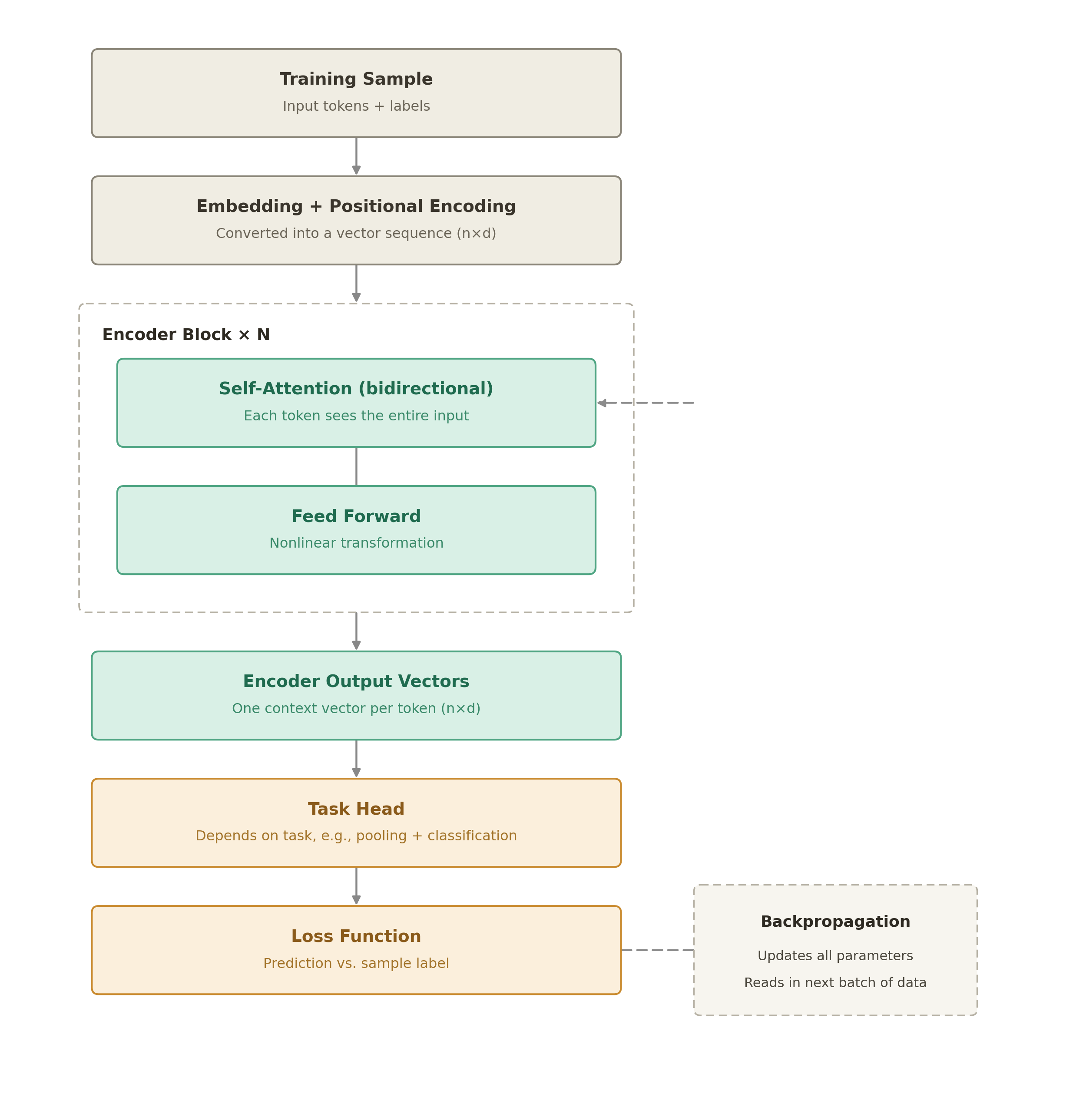
Training example: (这部电影太好看了 / “This movie was great”, label positive)
| Step | Module | Input | Output | Purpose |
|---|---|---|---|---|
| 1 | Training sample | Corpus | 这 部 电 影 太 好 看 了 (8 tokens) + label positive |
Input and label come as a pair |
| 2 | Embedding + positional encoding | 8 tokens | 8×d | Each token becomes a position-aware vector |
| 3 | Encoder block × N | 8×d | 8×d | Bidirectional self-attention + feed-forward, repeated N times |
| 4 | Encoder output vectors | 8×d | 8 contextual vectors | One vector per position |
| 5 | Task head | 8×d | Class probabilities (1×2) | Pool, then Linear + softmax; say early training gives [negative 0.40, positive 0.60] |
| 6 | Loss function | Class probabilities + label positive |
A scalar loss | Cross-entropy, −ln 0.60 ≈ 0.51 |
| 7 | Backpropagation | loss | Updated parameters | Gradients flow back through the task head, encoder, and embeddings — every parameter updates together |
| 8 | Next batch | Updated model | Back to step 1 | What loops here is training batches, not token-by-token generation |
Architecture during inference
Here’s the inference setup:
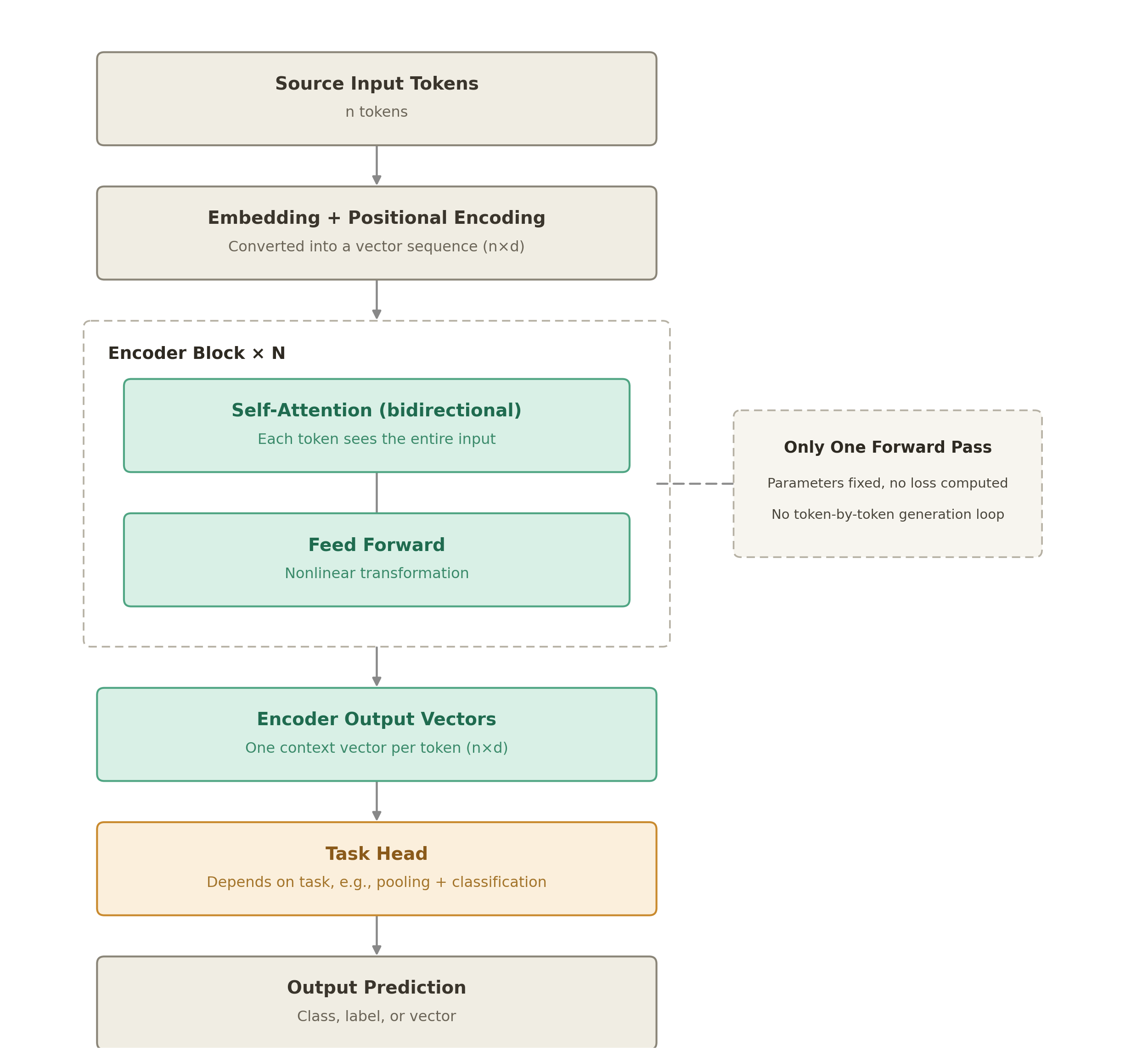
Input: 这部电影太好看了 (“This movie was great”)
| Step | Module | Input | Output | Purpose |
|---|---|---|---|---|
| 1 | Input tokens | A sentence | 这 部 电 影 太 好 看 了 (8 tokens) |
Split by character |
| 2 | Embedding + positional encoding | 8 tokens | 8×d | Each token becomes a position-aware vector |
| 3 | Encoder block × N | 8×d | 8×d | Bidirectional self-attention + feed-forward, repeated N times, fusing full-sentence context |
| 4 | Encoder output vectors | 8×d | 8 contextual vectors | One vector per position |
| 5 | Task head | 8×d | Class probabilities (1×2) | Pool into a single 1×d sentence vector, then Linear + softmax; say this gives [negative 0.03, positive 0.97] |
| 6 | Output prediction | Class probabilities | positive |
Take the highest-probability class |
Training adds a label, a loss function, and backpropagation on top of inference — inference itself is just a single forward pass.
The Decoder-only Transformer Architecture
The Transformer’s biggest application today — LLMs — are all decoder-only: ChatGPT, Claude, DeepSeek, you name it.
The architecture’s workflow actually matches how you use it directly. In a chat setting, for instance, the model generates a response to your input, and your input is simply the “already available” information.
A decoder-only model’s core mechanism is “continuation”: because of masked self-attention, it can only see what came before, and it generates based purely on that (which makes sense — continuation never needs “future” content anyway, since there isn’t any yet).
Architecture during training
Here’s the training setup for a decoder-only Transformer:
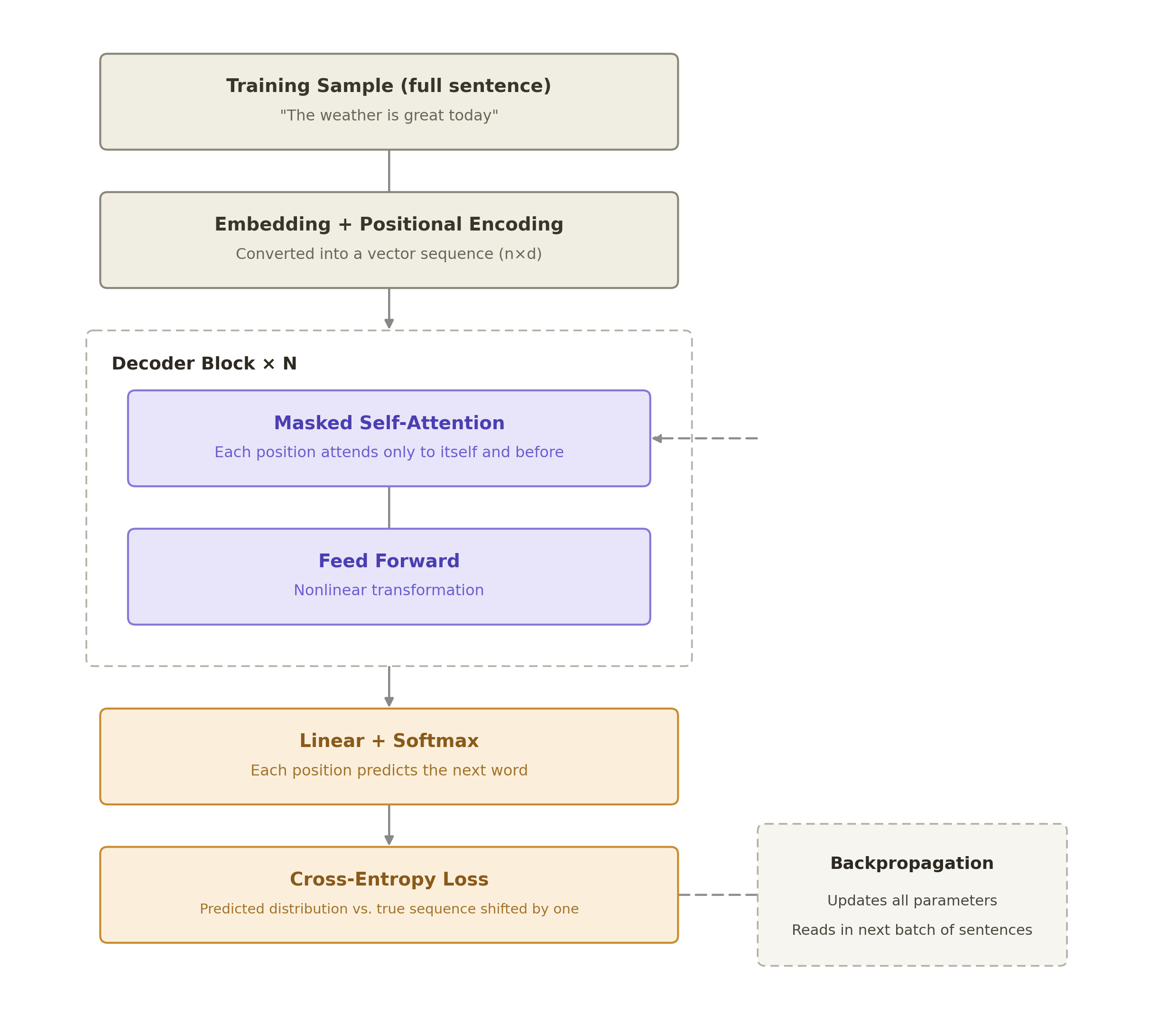
Example: training on “今天天气真好” (“The weather is really nice today”):
| Step | Module | Input | Output | Purpose |
|---|---|---|---|---|
| 1 | Training sample | Corpus | 今 天 天 气 真 好 (6 tokens) |
The whole sentence is fed in directly — no manual labeling needed, since the “label” is just the sequence shifted by one position |
| 2 | Embedding + positional encoding | 6 tokens | 6×d | Each token becomes a position-aware vector |
| 3 | Decoder block × N | 6×d | 6×d | Masked self-attention guarantees position $i$ can’t see position $i+1$ or beyond |
| 4 | Linear + softmax | 6×d (computed at every position) | 6 vocabulary probability distributions | Position “今” predicts the next word, position “天” (the first one) predicts the next word, and so on — all 6 positions computed in parallel |
| 5 | Cross-entropy loss | 6 predicted distributions + the actual next words | A scalar loss | e.g. position “今” should predict “天”, position “气” should predict “真”; sum or average the loss across all 6 positions |
| 6 | Backpropagation | loss | Updated parameters | Gradients flow back through the decoder and embeddings — all parameters update together |
| 7 | Next batch | Updated model | Back to step 1 | What loops here is training batches |
Architecture during inference
Here’s the inference setup for a decoder-only Transformer:
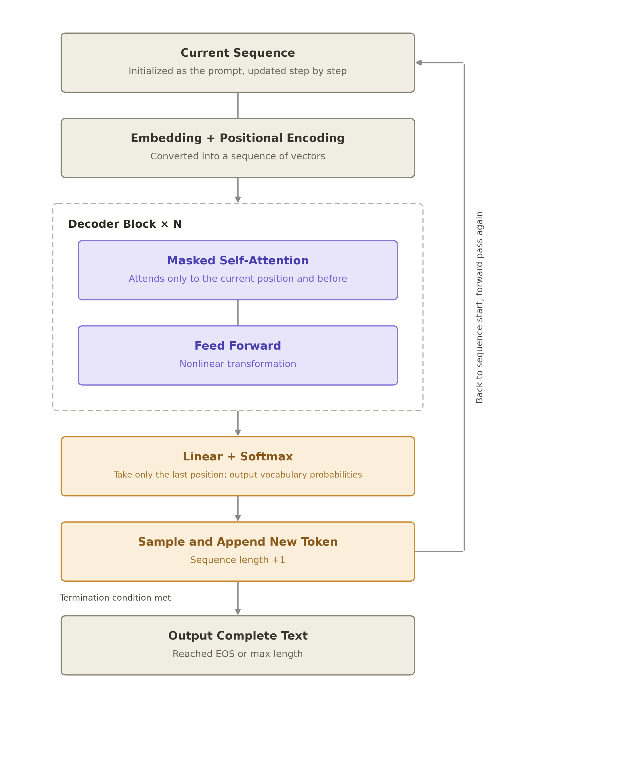
Continuing the same example: given the prompt “今天天气” (“The weather today”), continue it.
| Step | Module | Input | Output | Purpose |
|---|---|---|---|---|
| 1 | Current sequence | Prompt | 今 天 天 气 (4 tokens) |
Starting sequence |
| 2 | Embedding + positional encoding | 4 tokens | 4×d | Each token becomes a position-aware vector |
| 3 | Decoder block × N | 4×d | 4×d | Masked self-attention lets each position see only itself and everything to its left, repeated N times |
| 4 | Linear + softmax | Vector at the last position (1×d) | Vocabulary probabilities | Only the last position’s (“气”) vector is used to predict the next word — say this gives 真 0.6, 不 0.2, … |
| 5 | Sample and append | Vocabulary probabilities | 今 天 天 气 真 (5 tokens) |
Sample “真” and append it to the sequence |
| 6 | Back to step 2 | 今 天 天 气 真 |
Run a full forward pass again | The sequence grew longer, so every position is recomputed |
| 7 | Loop until done | Progressively longer sequence | 今天天气真好,适合出门 (“The weather is great today, good day to go out”) |
Stops on hitting EOS or a length limit |
Testing the Differences
I got curious how these three architectures actually stack up on the same task, so I had an AI write two experiments to find out.
Experiment 1: fill-in-the-blank by position
Setup
Using rule-generated synthetic sentences, blank out one position at a time, and have all three architectures (decoder-only / encoder-only / enc-dec) fill it in. Accuracy is bucketed by blank position — early, middle, late in the sentence — with a 3-gram prefix baseline thrown in for comparison.
Results
A single test run and its output (the synthetic animal used here is “frog”):
% .venv/bin/python demo.py frog
decoder: 420,413 params
encoder: 420,413 params
encdec: 949,565 params
==============================================================================
Original sentence: the mossy frog followed a shy deer in the pond .
pos   answer    Decoder-only   Encoder-only   Enc-Dec
pos1  mossy     rocky ✗        mossy          mossy          ← pure future info (determined only by the sentence-final location)
pos2  frog      frog           frog           frog
pos3  followed  followed       followed       followed
pos4  a         a              a              a
pos5  shy       shy            shy            shy            ← Decoder can infer this via the verb→object chain
pos6  deer      deer           deer           deer
pos7  in        in             in             in             ← Decoder can infer this via the subject→habitat chain
pos8  the       the            the            the
pos9  pond      pond           pond           pond
And the full-scale test run:
% .venv/bin/python eval.py
decoder: 420,413 params
encoder: 420,413 params
encdec: 949,565 params

===== Cloze Top-1 accuracy (by blank position) =====
bucket       decoder     encoder      encdec     unigram     3gram ceiling
early          49.0%       77.9%       78.2%        0.0%       34.6%
mid            80.3%       87.1%       86.8%        0.0%       79.6%
late           89.1%       90.1%       90.3%       33.0%       65.9%

===== Failure cases per model (top 5) =====

[decoder]
  (early) the swift cat [?] a mossy dog in the river .  | answer=followed pred=watched
  (early) the muddy [?] barked a lazy cat in the river .  | answer=dog pred=frog
  (mid) the quiet fox caught a [?] fox near the lake .  | answer=muddy pred=curious
  (late) the misty cat hunted a wild deer [?] the cave .  | answer=near pred=in
  (early) the muddy [?] chased a gentle mouse near the forest .  | answer=fox pred=frog

[encoder]
  (early) the swift cat [?] a mossy dog in the river .  | answer=followed pred=watched
  (mid) the quiet fox caught a [?] fox near the lake .  | answer=muddy pred=clever
  (late) the misty cat hunted a wild deer [?] the cave .  | answer=near pred=in
  (early) the rocky hawk [?] a hungry bear on the hill .  | answer=feared pred=spotted
  (mid) the rocky mouse sniffed a lazy [?] near the cave .  | answer=fox pred=cat

[encdec]
  (early) the swift cat [?] a mossy dog in the river .  | answer=followed pred=watched
  (mid) the quiet fox caught a [?] fox near the lake .  | answer=muddy pred=clever
  (early) the rocky hawk [?] a hungry bear on the hill .  | answer=feared pred=spotted
  (mid) the rocky mouse sniffed a lazy [?] near the cave .  | answer=fox pred=cat
  (late) the rocky fox spotted a sleepy frog in the [?] .  | answer=field pred=forest
Conclusion
Across a 5,000-example test set, bucketed by blank position, decoder-only accuracy climbs sharply from early to mid to late blanks (49% → 80% → 89%), while encoder-containing models stay consistently high across the board (78–90%). This shows that the earlier a blank appears in the sentence, the more costly it is to “not be able to see the future.”
Looking at this, beyond the well-known “context rot” problem, an LLM being too small is also a real liability — you need a model that’s appropriately sized.
Experiment 2: translating into an inverted pseudo-language
Encoder-only doesn’t get a seat at this table, since encoders can only do fill-in-the-blank, not open-ended generation tasks like translation. So this experiment only compares the full encoder-decoder framework against decoder-only.
Setup
Source and target are concatenated as source <SEP> target and fed to both decoder-only and enc-dec models. Under this setup, the decoder-only model also has full visibility into the source (the causal mask doesn’t block the input portion).
This lets us answer a specific question: “Is decoder-only, missing that extra piece, actually weaker than encoder-decoder?”
Results
Both hit 100% accuracy:
% .venv/bin/python translate_eval.py
encdec: 968,840 params
[encdec] exact-match accuracy 100.0%  word-level accuracy 100.0%
decoder: 439,688 params
[decoder] exact-match accuracy 100.0%  word-level accuracy 100.0%

===== Translation error examples =====

[encdec]

[decoder]

saved results/translate_main.png
But the speed difference was huge — roughly 5-6x:
| Enc-Dec | Decoder-only | |
|---|---|---|
| epoch 1 loss | 0.9009 | 1.2425 |
| epoch 3 loss | 0.0009 | 0.0040 |
| epoch 8 loss | 0.0001 | 0.0003 |
| Total time for 8 epochs | 19s | 111s |
| Per-epoch time (once stabilized) | ~2-2.5s | ~14s |
Conclusion
This confirms decoder-only isn’t inherently weaker than encoder-decoder. As long as the “future information” is folded into the unmasked prefix, it performs identically to enc-dec — and this is exactly how LLMs are actually used in practice.
Would be interesting to try something more complex in the future — my current hardware just isn’t up to it yet.